Project 3: Morphing Faces

# Set up
import cv2
import numpy as np
import os
import scipy.signal
from tqdm import tqdm
from matplotlib import pyplot as plt
import matplotlib
import cowsay
from glob import glob
import scipy

matplotlib.rcParams["figure.dpi"] = 100

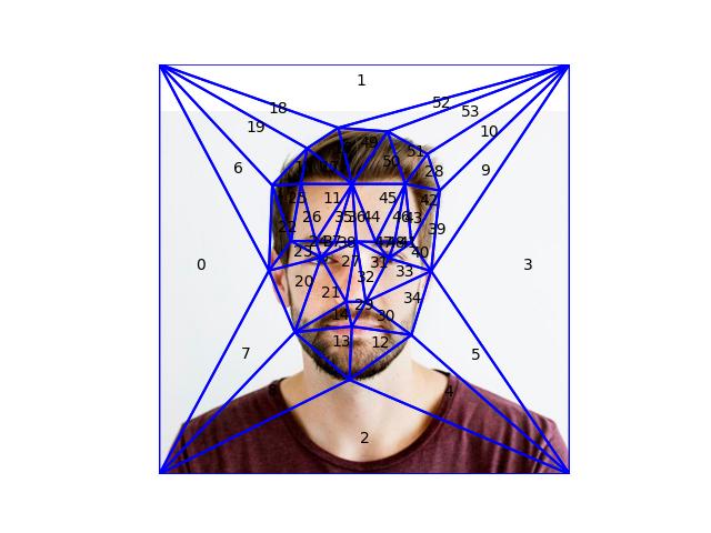
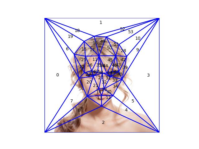
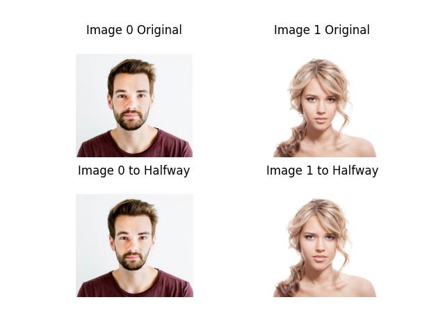
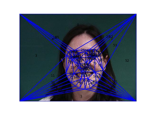
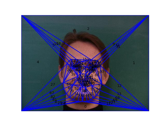
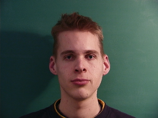
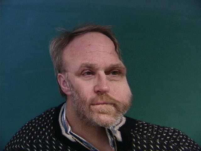
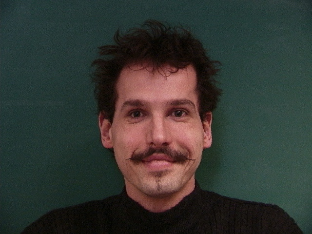
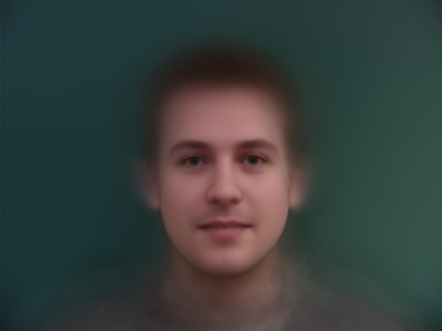
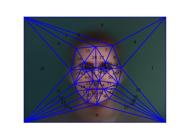
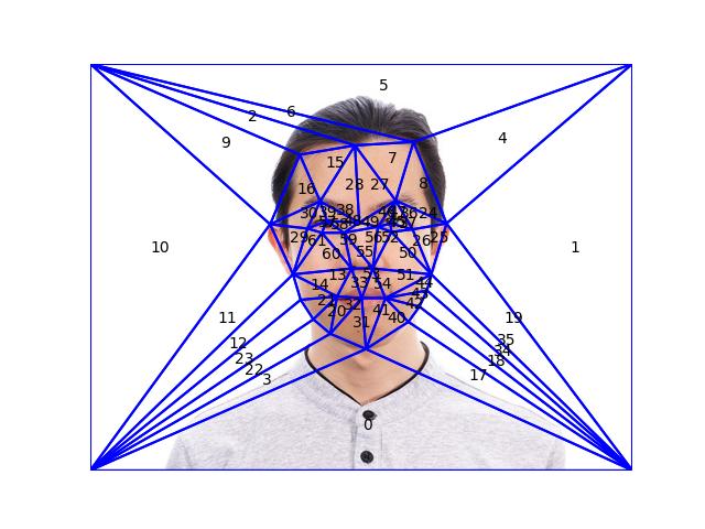
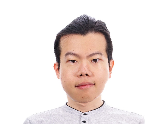
Part 1. Defining Correspondences

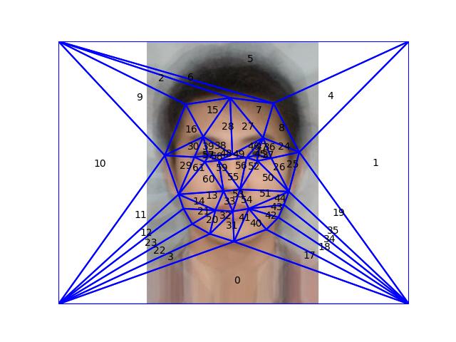
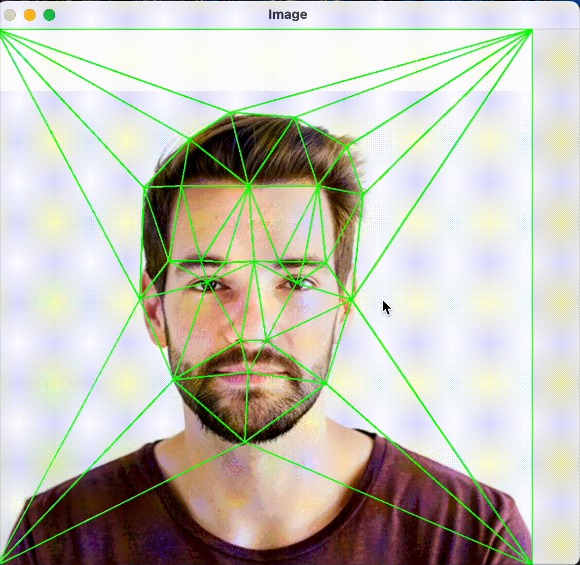
The correspondences have been defined using the label_img.py script, and we compute the Delaunay triangulation in this section. After adding the four corner points to ensure that the triangulation covers the entire image, we compute the triangular-mesh using Delaunay from scipy. Below we visualize the generated mesh overlaid on the images. The labels are the order of the triangles in the list, this is useful to check for any discrepencies in the mesh correspondence between the images so the morphing is more natural.

Part 2. Computing the "Mid-way Face"

To compute the Mid-way Face, we need to compute the correct location in pixel space for each of the corresponding points that we have defined. This is simply the average of the values, so for corresponding points in pixel space $(x_0, y_0)$ and $(x_1, y_1)$, we can compute the midway point's location $(x', y')$ with $$(x', y') = \frac{1}{2} ((x_0, y_0) + (x_1, y_1))$$

After computing the target, we then need to compute an affine transformation that maps all 3 points of the triangle from the source to the target. Then using this mapping, we compute the reverse map by inverting the homogeneous transformation matrix. Using this matrix, we can compute the pixels from the original image that should be mapped into the new transformed image. Floating point pixel spaces are rounded to the nearest integer value. Pixels that are beyond the boundaries of the original image are clipped.

Below we show the results of the halfway image. We can see the man's chin shifting to the left and the woman's chin shifting right to the man's position.

Part 3. The Morph Sequence

In this section, we add cross dissolve as well as incremental warping to smoothly transition from face A to face B. Let the completion ratio be $t \in [0, 1]$ and without loss of generality let us be morphing from image 0 to image 1, then at timestep $t$, the positions for each arbitrary point $(x', y')$ should be $$(x', y') = (1-t) (x_0, y_0) + t(x_1, y_1)$$

The opacities for image 0 should be $(1-t)$ and $t$ for image 1. When we put all of these together, we render the following video.

We observe that the transition looks natural and smooth

Part 4. The "Mean face" of a population

Compute the average face shape of the whole population or some subset of the population - say, all the old/young/white/asian/men/women etc. However, if you pick a subpopulation - make sure it contains enough faces for this to be interesting.

We first parse the ASF files that describe the correspondence of the points. We visualize a few triangulations to verify that the data is not corrupted.

To compute the average face of the Danes, it is similar to computing the midway face, but instead of 2 faces, it is every face in the dataset. Thus we can find

$$(x', y') = \sum_{i=1}^n \frac{1}{n} (x_i, y_i)$$

The average face is then the average of all the warped faces. The warps range from fairly normal to relatively bizarre depending on where the person in frame is looking and whether their head is tilted.

We find that our final result does look fairly resonable:

It was difficult to replicate the labels of the IMM dataset, so manual relabeling was required to achieve morphing from my face to the average Dane and vice versa.

With the correspondences and triangulations properly defined, we can compute morphs.

Part 5. Caricatures: Extrapolating from the mean

For this section, we compare the extrapolation from the mean of the Danes and the mean of the Chinese. The mean of the Chinese is similarly labelled.

For this computation, we first find the difference between my face's coordinates and the mean's, and then add it to my coordinates, thus increasing my deviation from the mean. Thus if points on my photo are $(x_0, y_0)$ and $(x_m, y_m)$ for the mean, we can find $$(x', y') = 2 (x_m, y_m) - (x_0, y_0)$$

Following this computation, we create the following images:

extrapolated_from_chinese = plt.imread("output/extrapolated_from_chinese.jpg")
extrapolated_from_dane = plt.imread("output/extrapolated_from_dane.jpg")

fig, ax = plt.subplots(1, 2, figsize=(10, 5))
ax[0].imshow(extrapolated_from_chinese)
ax[0].axis("off")
ax[0].set_title("From Chinese")
ax[1].imshow(extrapolated_from_dane)
ax[1].axis("off")
ax[1].set_title("From Dane")

Text(0.5, 1.0, 'From Dane')

Bells and Whistles

PCA Basis

For this section, we first convert the images to black and white for numerical stability. Then we compute a PCA basis for all the un-warped images, and then we perform the warping for the average face as normal.

We first test our low-rank approximation using the top 100 singular values.

As expected, there are quite a few artifacts due to the fact that in some images, people are looking in different directions, making it difficult to represent this variety in only 100 vectors.

We then compute the mean face using the warp algorithm as described above, and we observe that the result is remarkably good.

We now compare it side by side with the original method.

color_mean = plt.imread("output/average_face.jpg")
low_rank = plt.imread("output/low_rank_mean_face.jpg")

fig, ax = plt.subplots(1, 2, figsize=(10, 5))
ax[0].imshow(color_mean)
ax[0].axis("off")
ax[0].set_title("Color Mean")
ax[1].imshow(low_rank, cmap="gray")
ax[1].axis("off")
ax[1].set_title("Low Rank Mean")

Text(0.5, 1.0, 'Low Rank Mean')

This demonstrates that performing the warp in PCA space may have beneficial effects since we need to store less data for each of the images due to the low rank projection.

Drag and Drop Live Editor

We implemented a editor that reads an image and the corresponding labels, and computes a Delaunay hull to enable live morphing by dragging and dropping the points on the image. We present a video of the tool as well as the final result.

Diamond man is coming to get you.