Project 2: Fun with Filters and Frequencies!

# Set up
import cv2
import numpy as np
import os
import scipy.signal
import tqdm
from matplotlib import pyplot as plt
import matplotlib
import cowsay
import scipy
matplotlib.rcParams["figure.dpi"] = 500

Part 1: Fun with Filters

Part 1.1: Finite Difference Operator

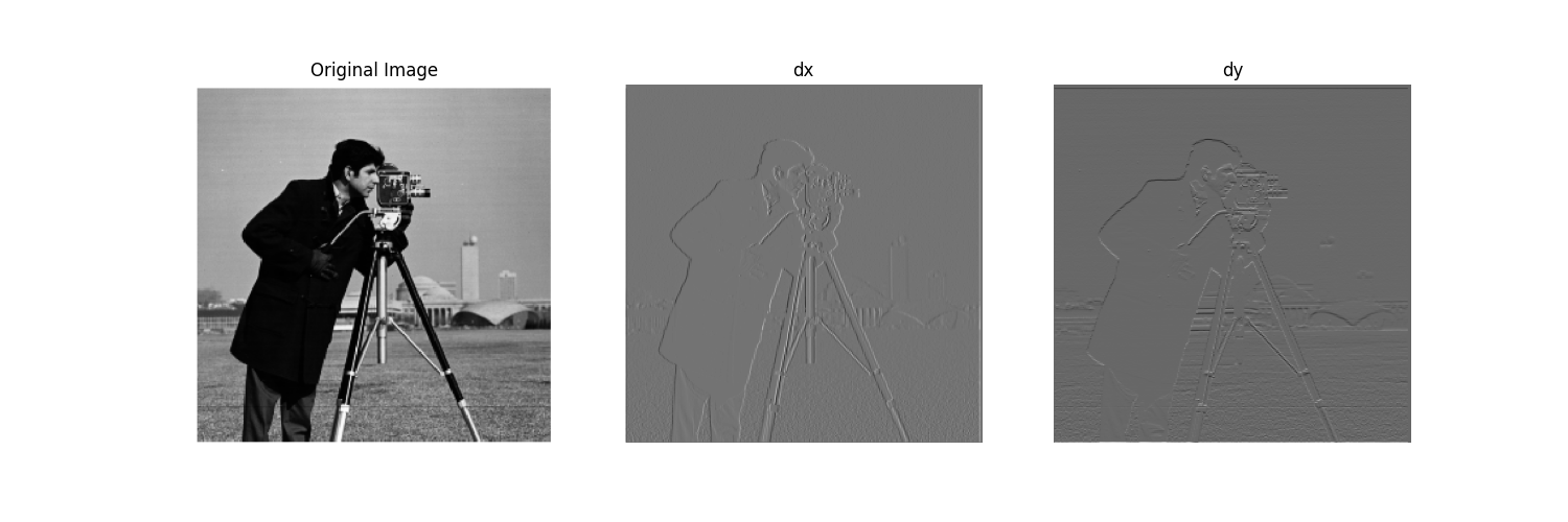
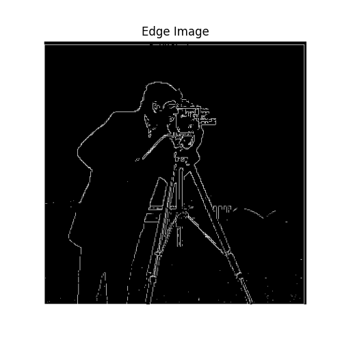
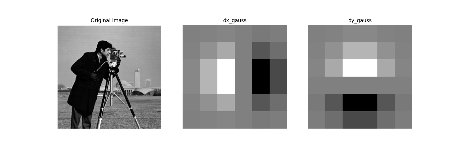
In this section, we compute the gradient of the image in the $x$ and $y$ directions. Since the gradient is simply the rate of change and images are discretized in pixels, the filters $\begin{bmatrix} 1 & -1\\ \end{bmatrix}$ and $\begin{bmatrix} 1\\ -1 \end{bmatrix}$ compute the partial derivatives in the x and y directions respectively. When we convolve over the whole image $I$, we get $\frac{\partial I}{\partial x}$ and $\frac{\partial I}{\partial y}$, thus we can compute the magnitude of the gradient: $$||\nabla|| = \sqrt{(\frac{\partial I}{\partial x})^2 + (\frac{\partial I}{\partial y})^2}$$

Part 1.2: Derivative of Gaussian (DoG) Filter

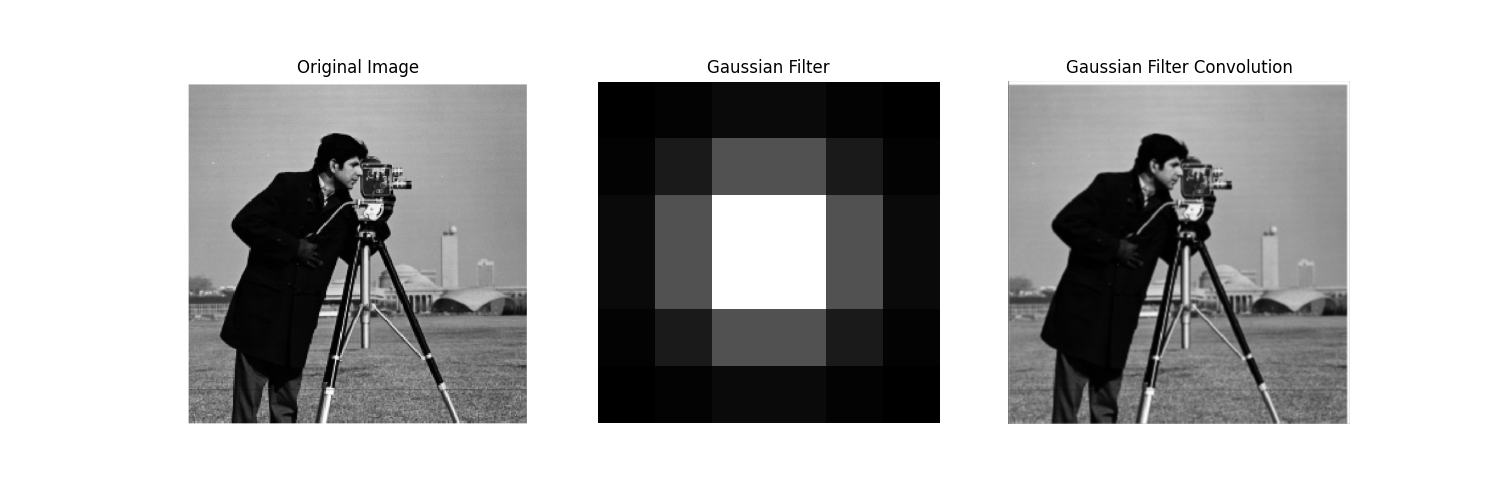
After this filtering, the edges are smoother and we do not see as many noise (gaps in the trace).

What differences do you see?

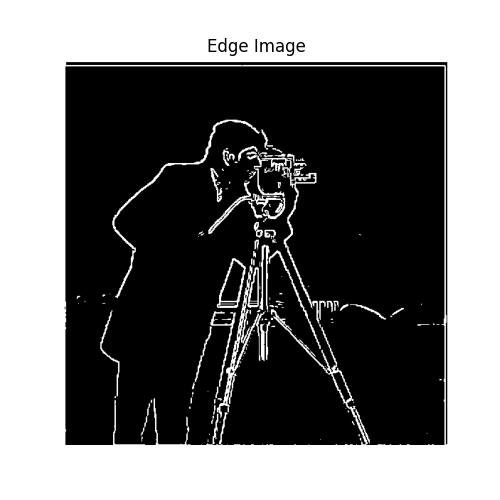
When binarizing, the threshold is much easier to find and the resulting edge image is more complete and consistent. The gaussian edge gets the vast majority of the camera man as well as his camera and tripod, whereas directly using dx, dy will only get parts of it with a higher threshold and a lot of noise with a lower one.

We then use the gaussian filter pre-convovled with dx and dy filters.

Verify that you get the same result as before

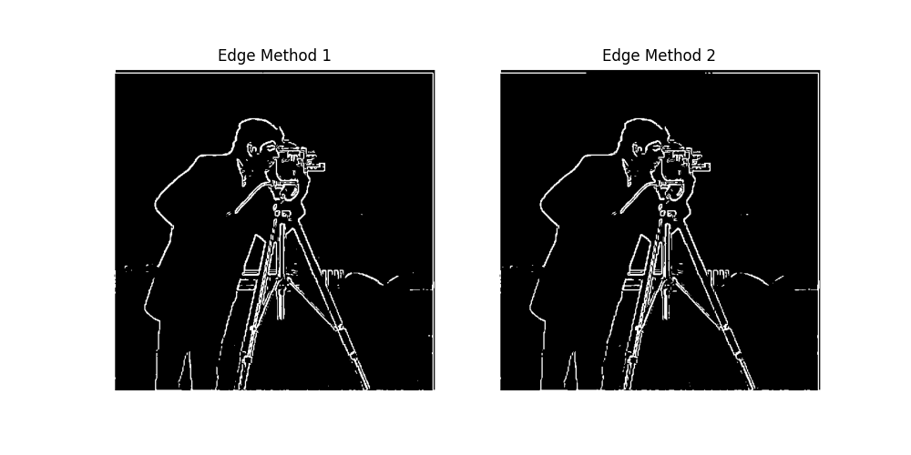
The last visualization confirms this.

Part 2: Fun with Frequencies

Part 2.1: Image "Sharpening"

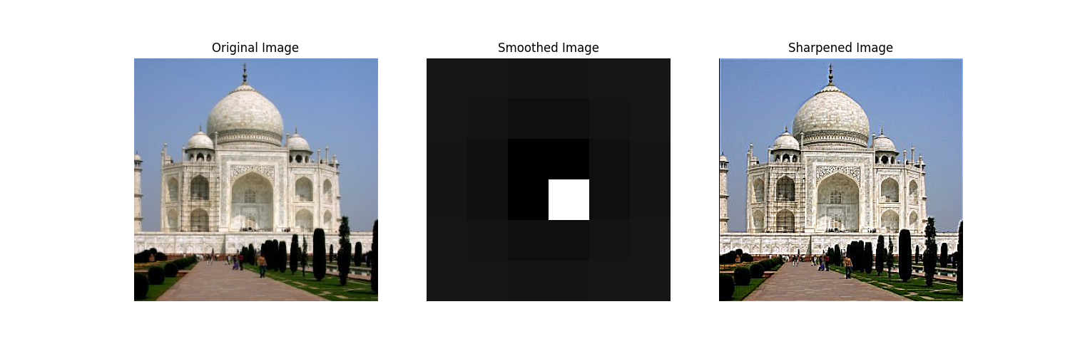
We first obeserve the taj mahal picturend then use the laplacian sharpen filter (visualized) to convolve. This produces an image with emphasized edges.

Blurring and Resharpening

We take the Arcane poster and first blur it with the Gaussian filter and then sharpen it using the method above.

Oberservation

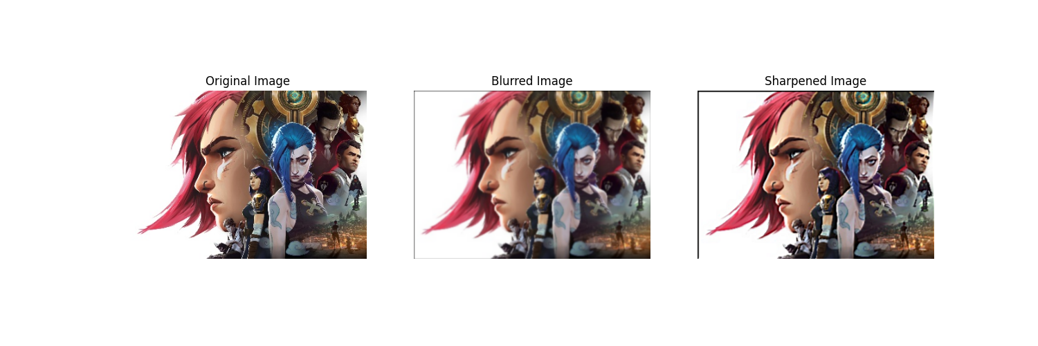
We observe that by blurring and then sharpening, we are able to recover some of the higher frequencies such as Vi's hair, but this process loses a lot of information such as the highlights on Mel's shoulder plate. This is likely due to the fact that some image details exist across mutliple frequencies so we are able to retrieve some of it from the blurred images but some are not. In this case we would not be able to recover these information from the blurred image.

2.3 Hybrid Images

Fourier Analysis

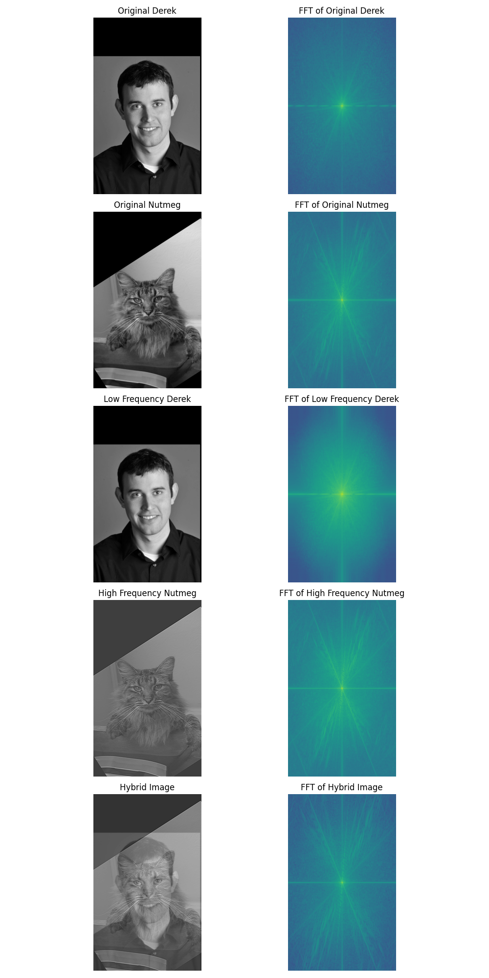
We observe the aligned gray-scale images as well as the fourier frequencies. When blurred, we expect Derek's high frequencies go down, and we observe that the frequencies on the edges are lower. When filtered, Nutmeg's low frequencies are lower. When we combine them, we get a hybrid image of Derek and Nutmeg.

Additional Hybrids

For this, we merged Jinx and Vi, and Derek and a capybara. Code below is visualization only and contains no computation.

jinx = plt.imread("data/jinx.jpg")
vi = plt.imread("data/vi.jpg")
jinx_vi = plt.imread("data/hybrid_jv.jpg")

fig, ax = plt.subplots(1, 3, figsize=(15, 5))
ax[0].imshow(jinx)
ax[0].axis("off")
ax[0].set_title("Jinx")
ax[1].imshow(vi)
ax[1].axis("off")
ax[1].set_title("Vi")
ax[2].imshow(jinx_vi, cmap="gray")
ax[2].axis("off")
ax[2].set_title("Jinx-Vi")

Text(0.5, 1.0, 'Jinx-Vi')

Failure Case

Below is a failure case and the result looks very strange. This is most likely due to the fact that Derek does not share a lot of features with the capybara and the frequencies clash with each other.

derek = plt.imread("data/DerekPicture.jpg")
capy = plt.imread("data/capybara.jpg")
jinx_vi = plt.imread("data/hybrid_dc.jpg")

fig, ax = plt.subplots(1, 3, figsize=(15, 5))
ax[0].imshow(derek)
ax[0].axis("off")
ax[0].set_title("Derek")
ax[1].imshow(capy)
ax[1].axis("off")
ax[1].set_title("Capybara")
ax[2].imshow(jinx_vi, cmap="gray")
ax[2].axis("off")
ax[2].set_title("Derek-bara")

Text(0.5, 1.0, 'Derek-bara')

2.4 Gaussian and Laplacian Stack

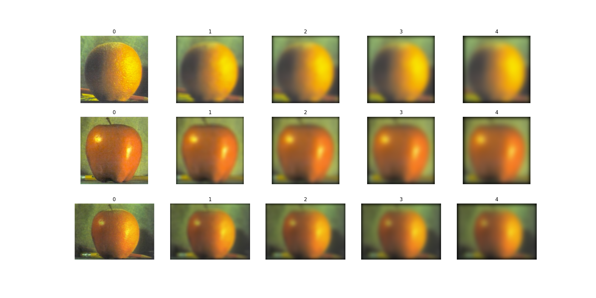
We first create the blurred orange, apple, and oraple stack.

.

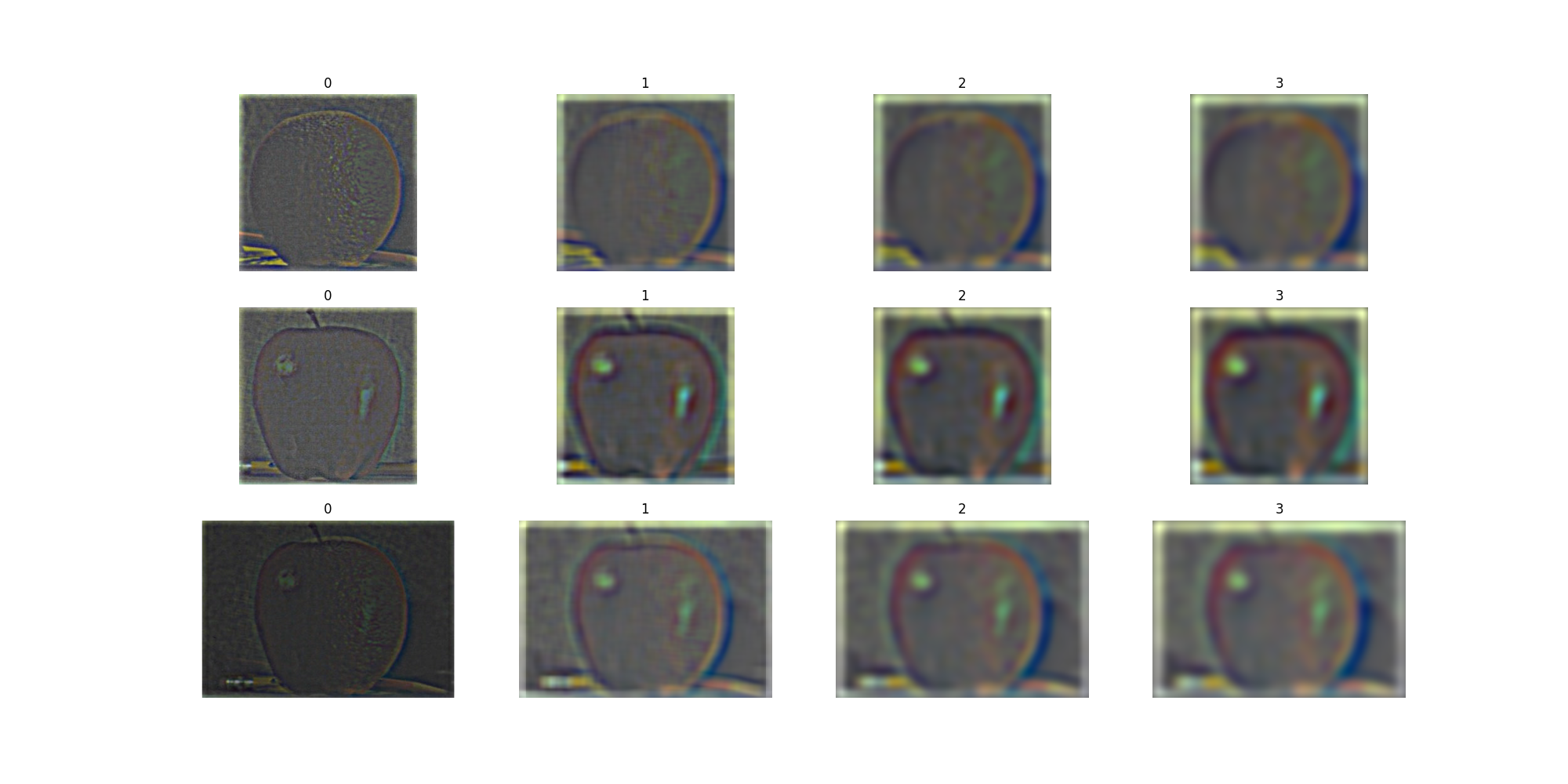
The first layer is the unblurred version. We then compute the difference between each layer to get the Laplacian Stack.

2.5 Multiresolution Blending

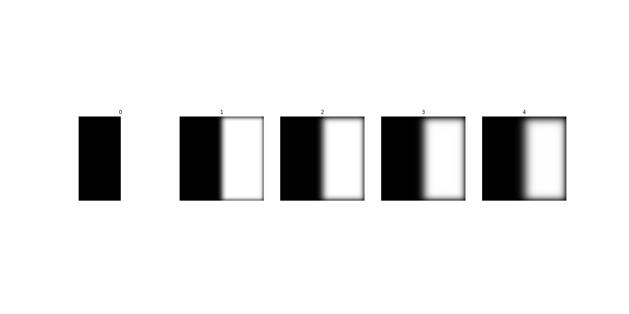
In order to combine these different resolutions, we first also compute the different masks at these resolutions. The computation is similar: create a mask stack by iteratively blurring the mask. In this case, the mask is simply a stepper function, with half of the image being 1 and the other half 0. Below we visualize this blurring:

Let the 2 images be $A$, $B$. Let the Gaussian stack be $G_{Ai}$ and $G_{Bi}$, with $i$ being the level of the stack.Let the mask stacks be $M_{i}$. Similarly let the Laplacian stack be denoted by $L_{Ai}$ and $L_{Bi}$.

During computation, we go from the highest level of the stack down to 0. At each level $i$, we can compute the blended image $B_{i-1} = B{i} + M_{i} * L_{Ai} + (1-M_{i})*L_{Bi}$. The starting image $B_{\text{max}}$ is defined as $B_{\text{max}} = M_{\text{max}} * G_{A\text{max}} + (1-M_{\text{max}})*L_{B\text{max}}$. Our starting image is simply the masked blends of the last layers of the gaussian stack and we iteratively add the masked blends of the laplacian stack.

Using this method, we produce the following iamge, which is quite similar to the original.

original_orple = plt.imread("data/orple.jpg")
my_orple = plt.imread("data/my_orple.jpg")

fig, ax = plt.subplots(1, 2, figsize=(10, 5))
ax[0].imshow(original_orple)
ax[0].axis("off")
ax[0].set_title("Original Orple")
ax[1].imshow(my_orple, cmap="gray")
ax[1].axis("off")
ax[1].set_title("My Orple")

Text(0.5, 1.0, 'My Orple')

We continue experimenting with a seam between the top and bottom halves of the image.

banana = plt.imread("data/banana.jpg")
tree = plt.imread("data/tree.jpg")
banana_tree = plt.imread("data/banana_tree.jpg")

fig, ax = plt.subplots(1, 3, figsize=(15, 5))
ax[0].imshow(banana)
ax[0].axis("off")
ax[0].set_title("Banana")
ax[1].imshow(tree)
ax[1].axis("off")
ax[1].set_title("Tree")
ax[2].imshow(banana_tree, cmap="gray")
ax[2].axis("off")
ax[2].set_title("Banana-Tree")

Text(0.5, 1.0, 'Banana-Tree')

We finish by bringing the capybara back with a more suitable blending target. The mask is generated with photoshop.

capybara = plt.imread("data/big_capy.jpg",)
tiger = plt.imread("data/tiger.jpg")
capy_mask = plt.imread("data/mask.jpg")
tiger_bara = plt.imread("data/tiger_bara.jpg")

fig, ax = plt.subplots(1, 4, figsize=(20, 5))
ax[0].imshow(capybara)
ax[0].axis("off")
ax[0].set_title("Capybara")
ax[1].imshow(capy_mask, cmap="gray")
ax[1].axis("off")
ax[1].set_title("Mask")
ax[2].imshow(tiger)
ax[2].axis("off")
ax[2].set_title("Tiger")
ax[3].imshow(tiger_bara)
ax[3].axis("off")
ax[3].set_title("Tiger-bara")

Text(0.5, 1.0, 'Tiger-bara')