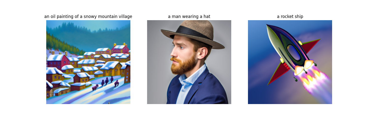
In this problem set you will play around with diffusion models, implement diffusion sampling loops, and use them for other tasks such as inpainting and creating optical illusions.
We are going to use the DeepFloyd IF diffusion model. DeepFloyd is a two stage model trained by Stability AI. The first stage produces images of size $64 \times 64$ and the second stage takes the outputs of the first stage and generates images of size $256 \times 256$. We provide upsampling code at the very end of the notebook, though this is not required in your submission.
Before using DeepFloyd, you must accept its usage conditions. To do so:
The objects instantiated above, stage_1
and
stage_2
, already contain code to allow us to sample
images using these models. Read the code below carefully
(including the comments) and then run the cell to generate some
images. Play around with different prompts and
num_inference_steps
.
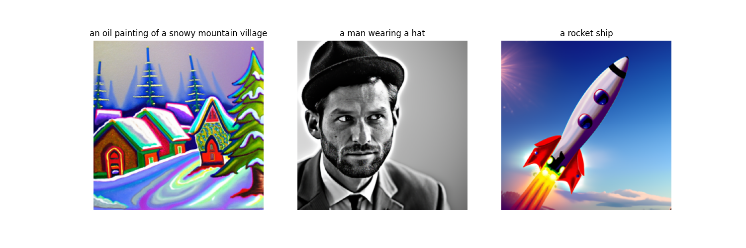
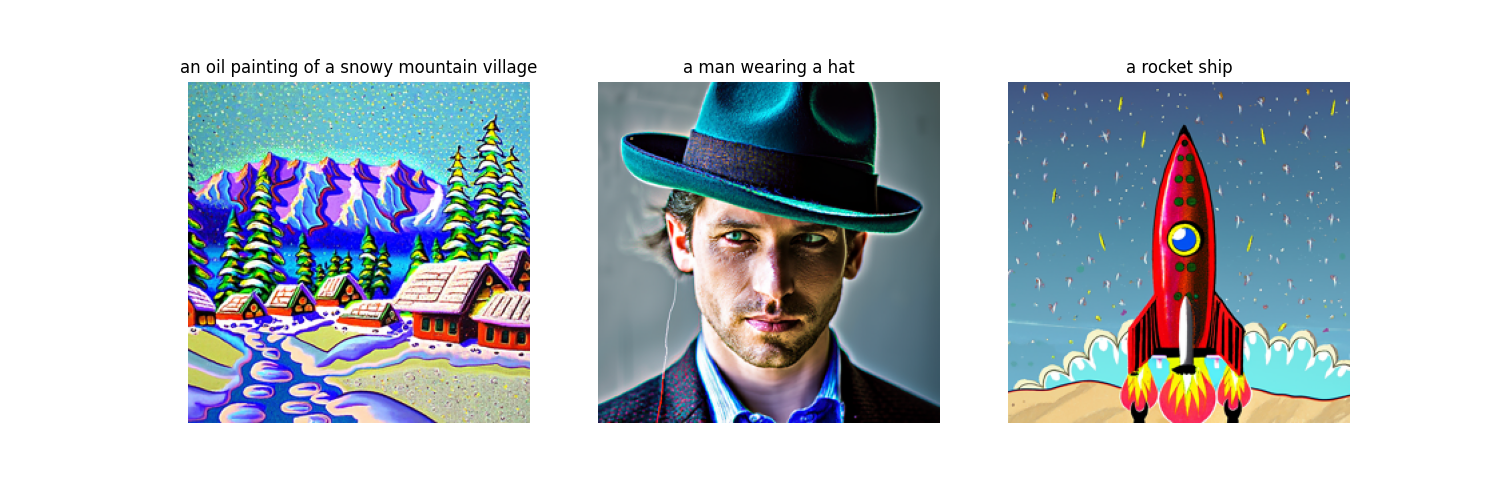
This is the generated image with 10 inference steps.
With 20 steps
With 100 steps
The image quality seems to increase as the number of inference steps increases. The images have more details and are less blurry.
In this part of the problem set, you will write your own "sampling loops" that use the pretrained DeepFloyd denoisers. These should produce high quality images such as the ones generated above.
You will then modify these sampling loops to solve different tasks such as inpainting or producing optical illusions.
Starting with a clean image, $x_0$, we can iteratively add noise to an image, obtaining progressively more and more noisy versions of the image, $x_t$, until we're left with basically pure noise at timestep $t=T$. When $t=0$, we have a clean image, and for larger $t$ more noise is in the image.
A diffusion model tries to reverse this process by denoising the image. By giving a diffusion model a noisy $x_t$ and the timestep $t$, the model predicts the noise in the image. With the predicted noise, we can either completely remove the noise from the image, to obtain an estimate of $x_0$, or we can remove just a portion of the noise, obtaining an estimate of $x_{t-1}$, with slightly less noise.
To generate images from the diffusion model (sampling), we start with pure noise at timestep $T$ sampled from a gaussian distribution, which we denote $x_T$. We can then predict and remove part of the noise, giving us $x_{T-1}$. Repeating this process until we arrive at $x_0$ gives us a clean image.
For the DeepFloyd models, $T = 1000$.
The exact amount of noise added at each step is dictated by noise
coefficients, $\bar\alpha_t$, which were chosen by the people who
trained DeepFloyd. Run the cell below to create
alphas_cumprod
, which retrieves these coefficients
and downloads a test image that we will work with.
Disclaimer about equations: Colab cannot correctly render the math equations below. Please cross-reference them with the part A webpage to make sure that you're looking at the fully correct equation.
A key part of diffusion is the forward process, which takes a clean image and adds noise to it. In this part, we will write a function to implement this. The forward process is defined by:
$$ q(x_t | x_0) = N(x_t ; \sqrt{\bar\alpha_t} x_0, (1 - \bar\alpha_t)\mathbf{I})\tag{1}$$which is equivalent to computing $$ x_t = \sqrt{\bar\alpha_t} x_0 + \sqrt{1 - \bar\alpha_t} \epsilon \quad \text{where}~ \epsilon \sim N(0, 1) \tag{2}$$
That is, given a clean image $x_0$, we get a noisy image $ x_t $ at timestep $t$ by sampling from a Gaussian with mean $ \sqrt{\bar\alpha_t} x_0 $ and variance $ (1 - \bar\alpha_t) $. Note that the forward process is not just adding noise -- we also scale the image.
Below we show the images at different noise levels:
Let's try to denoise these images using classical methods. Again, take noisy images for timesteps [250, 500, 750], but use Gaussian blur filtering to try to remove the noise. Getting good results should be quite difficult, if not impossible.
We confirm this from the figures shown above. The Gaussian Cleaned is not legible at 750.
Now, we'll use a pretrained diffusion model to denoise. The actual
denoiser can be found at stage_1.unet
. This is a UNet
that has already been trained on a very, very large
dataset of $(x_0, x_t)$ pairs of images. We can use it to recover
Gaussian noise from the image. Then, we can remove this noise to
recover (something close to) the original image. Note: this UNet
is conditioned on the amount of Gaussian noise by taking timestep
$t$ as additional input.
Because this diffusion model was trained with text conditioning,
we also need a text prompt embedding. We provide the embedding for
the prompt "a high quality photo"
for you
to use. Later on, you can use your own text prompts.
The estimated images are shown above, we observe that the denoising process blurs the images, and some details are removed in this one-step process.
In part 1.3, you should see that the denoising UNet does a much better job of projecting the image onto the natural image manifold, but it does get worse as you add more noise. This makes sense, as the problem is much harder with more noise!
But diffusion models are designed to denoise iteratively. In this part we will implement this.
In theory, we could start with noise $x_{1000}$ at timestep $T=1000$, denoise for one step to get an estimate of $x_{999}$, and carry on until we get $x_0$. But this would require running the diffusion model 1000 times, which is quite slow (and costs $$$).
It turns out, we can actually speed things up by skipping steps. The rationale for why this is possible is due to a connection with differential equations. It's a tad complicated, and out of scope for this course, but if you're interested you can check out this excellent article.
To skip steps we can create a list of timesteps that we'll call
strided_timesteps
, which will be much shorter than
the full list of 1000 timesteps.
strided_timesteps[0]
will correspond to the noisiest
image (and thus the largest $t$) and
strided_timesteps[-1]
will correspond to a clean
image (and thus $t = 0$). One simple way of constructing this list
is by introducing a regular stride step (e.g. stride of 30 works
well).
On the i
th denoising step we are at $ t = $
strided_timesteps[i]
, and want to get to $ t' =$
strided_timesteps[i+1]
(from more noisy to less
noisy). To actually do this, we have the following formula:
$ x_{t'} = \frac{\sqrt{\bar\alpha_{t'}}\beta_t}{1 - \bar\alpha_t} x_0 + \frac{\sqrt{\alpha_t}(1 - \bar\alpha_{t'})}{1 - \bar\alpha_t} x_t + v_\sigma$
where:
alphas_cumprod
, as
explained above.
The $v_\sigma$ is random noise, which in the case of DeepFloyd is
also predicted. The process to compute this is not very important
for us, so we supply a function, add_variance
, to do
this for you.
You can think of this as a linear interpolation between the signal and noise:
For more information, see equations 6 and 7 of the DDPM paper. Be careful about bars above the alpha! Some have them and some do not.
Please first create the list strided_timesteps
. You
should start at timestep 990, and take step sizes of size 30 until
you arrive at 0. After completing the problem set, feel free to
try different "schedules" of timesteps.
Please also implement the function
iterative_denoise(image, i_start)
, which takes a
noisy image image
, as well as a starting index
i_start
. The function should denoise an image
starting at timestep timestep[i_start]
, applying the
above formula to obtain an image at timestep
t' = timestep[i_start + 1]
, and repeat iteratively
until we arrive at a clean image.
Please add noise to the test image im
to timestep
timestep[10]
and display this image. Then run the
iterative_denoise
function on the noisy image, with
i_start = 10
, to obtain a clean image and display it.
Please display every 5th image of the denoising loop. Compare this
to the "one-step" denoising method from the previous
section, and to gaussian blurring.
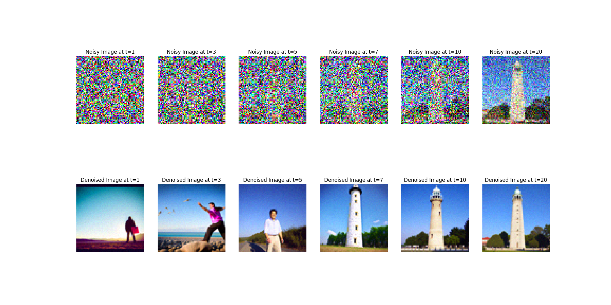
We demonstrate a single denoising trajectory.
We observe that the predicted clean image has increasingly less noise and more details begin to appear as the iterations get higher.
We further observe that the iteratively denoised image has more details than a single step denoised image.
In part 1.4, we use the diffusion model to denoise an image.
Another thing we can do with the
iterative_denoise
function is to generate images from
scratch. We can do this by setting i_start = 0
and
passing in random noise. This effectively denoises pure noise.
Please do this, and show 5 results of
"a high quality photo"
.
The images seem to be rather peculiar, and not very representative of real photos.
You may have noticed that some of the generated images in the prior section are not very good. In order to greatly improve image quality (at the expense of image diversity), we can use a technique called Classifier-Free Guidance.
In CFG, we compute both a noise estimate conditioned on a text prompt, and an unconditional noise estimate. We denote these $\epsilon_c$ and $\epsilon_u$. Then, we let our new noise estimate be
$$\epsilon = \epsilon_u + \gamma (\epsilon_c - \epsilon_u) \tag{4}$$where $\gamma$ controls the strength of CFG. Notice that for $\gamma=0$, we get an unconditional noise estimate, and for $\gamma=1$ we get the conditional noise estimate. The magic happens when $\gamma > 1$. In this case, we get much higher quality images. Why this happens is still up to vigorous debate. For more information on CFG, you can check out this blog post.
Please implement the iterative_denoise_cfg
function,
identical to the iterative_denoise
function but using
classifier-free guidance. To get an unconditional noise estimate,
we can just pass an empty prompt embedding to the diffusion model
(the model was trained to predict an unconditional noise estimate
when given an empty text prompt).
Before, we used "a high quality photo"
as a
"null" condition. Now, we will use the actual
""
null prompt for unconditional guidance
for CFG. In the later part, you should always use
""
null prompt for unconditional guidance
and use "a high quality photo"
for
unconditional generation.
The generated images are now much more similar to real photos.
In part 1.4, we take a real image, add noise to it, and then denoise. This effectively allows us to make edits to existing images. The more noise we add, the larger the edit will be. This works because in order to denoise an image, the diffusion model must to some extent "hallucinate" new things -- the model has to be "creative." Another way to think about it is that the denoising process "forces" a noisy image back onto the manifold of natural images.
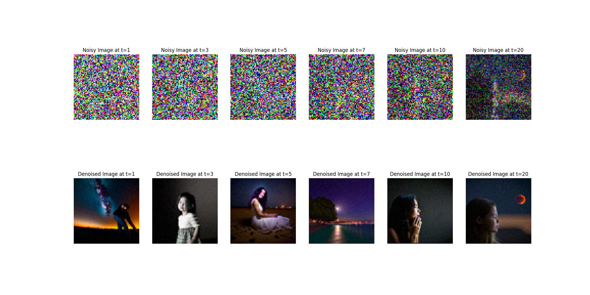
Here, we're going to take the original test image, noise it a little, and force it back onto the image manifold without any conditioning. Effectively, we're going to get an image that is similar to the test image (with a low-enough noise level). This follows the SDEdit algorithm.
To start, please run the forward process to get a noisy test
image, and then run the
iterative_denoise_cfg
function using a starting index
of [1, 3, 5, 7, 10, 20] steps and show the results, labeled with
the starting index. You should see a series of "edits"
to the original image, gradually matching the original image
closer and closer.
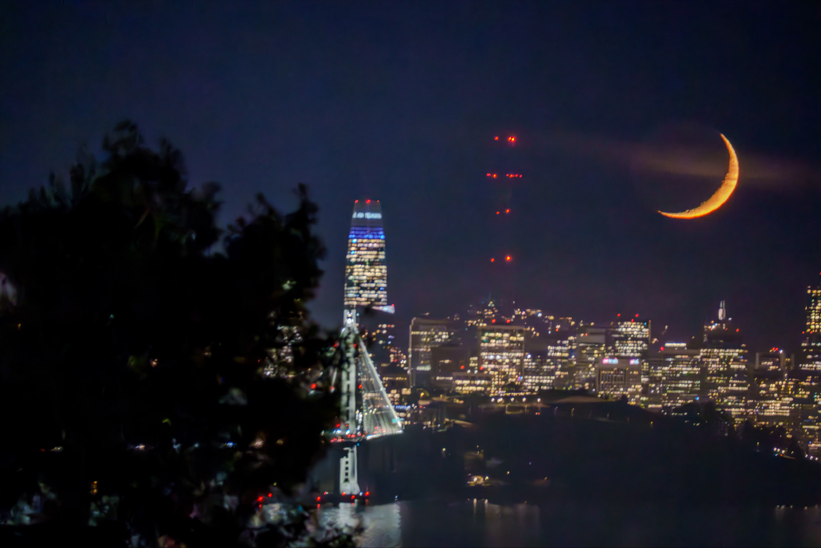
For our test image, we are using this photo of the Salesforce Tower that I took.
We notice that it doesn't recover the tower, but hallucinates a child. This is possibly due to the tower being quite out of focus and the moon being the most important subject in the image.
This procedure works particularly well if we start with a nonrealistic image (e.g. painting, a sketch, some scribbles) and project it onto the natural image manifold.
Please experiment by starting with hand-drawn or other non-realistic images and see how you can get them onto the natural image manifold in fun ways.
We provide you with 2 ways to provide inputs to the model:
Please find an image from the internet and apply edits exactly as above. And also draw your own images, and apply edits exactly as above. Feel free to copy the prior cell here. For drawing inspiration, you can check out the examples on this project page.
For our image, we used the provided avocado clip art. The model turned it into something that looked like a tangerine.
For the hand drawn images, we used a hand drawn rat and bird. The results were quite impressive, especially after upsampling.
Interestingly, the model gave a rat 2 tails at t=10, but performed better with birds, and both prompts looked fairly realistic at t=5
We can use the same procedure to implement inpainting (following the RePaint paper). That is, given an image $x_{orig}$, and a binary mask $\bf m$, we can create a new image that has the same content where $\bf m$ is 0, but new content wherever $\bf m$ is 1.
To do this, we can run the diffusion denoising loop. But at every step, after obtaining $x_t$, we "force" $x_t$ to have the same pixels as $x_{orig}$ where $\bf m = 0$, i.e.:
$ x_t \leftarrow \textbf{m} x_t + (1 - \textbf{m}) \text{forward}(x_{orig}, t) $
Essentially, we leave everything inside the edit mask alone, but we replace everything outside the edit mask with our original image -- with the correct amount of noise added for timestep $t$.
For our own images, we used a photo of a flower and a squirrel.
Interstingly, the model was reasonably successfuly at filling in the center of the flower, but hallucinated an entire person on the right half of the squirrel image.
Now, we will do the same thing as the previous section, but guide
the projection with a text prompt. This is no longer pure
"projection to the natural image manifold" but also adds
control using language. This is simply a matter of changing the
prompt from "a high quality photo"
to any
of the precomputed prompts we provide you (if you want to use your
own prompts, see appendix).
The spaceship - campanile
The dragon - squirrel
The dress - flower
We find that the model was exceptional at the spaceship and the dragon, but the dress photos were a bit lackluster
In this part, we are finally ready to implement
Visual Anagrams
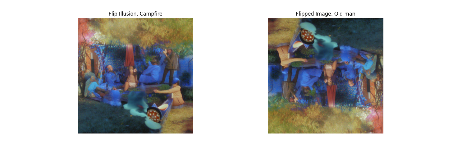
and create optical illusions with diffusion models. In this part,
we will create an image that looks like
"an oil painting of people around a campfire"
, but when flipped upside down will reveal
"an oil painting of an old man"
.
To do this, we will denoise an image $x_t$ at step $t$ normally
with the prompt
"an oil painting of an old man"
, to obtain
noise estimate $\epsilon_1$. But at the same time, we will flip
$x_t$ upside down, and denoise with the prompt
"an oil painting of people around a campfire"
, to get noise estimate $\epsilon_2$. We can flip $\epsilon_2$
back, to make it right-side up, and average the two noise
estimates. We can then perform a reverse diffusion step with the
averaged noise estimate.
The full algorithm will be:
$ \epsilon_1 = \text{UNet}(x_t, t, p_1) $
$ \epsilon_2 = \text{flip}(\text{UNet}(\text{flip}(x_t), t, p_2))$
$ \epsilon = (\epsilon_1 + \epsilon_2) / 2 $
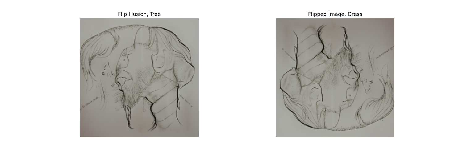
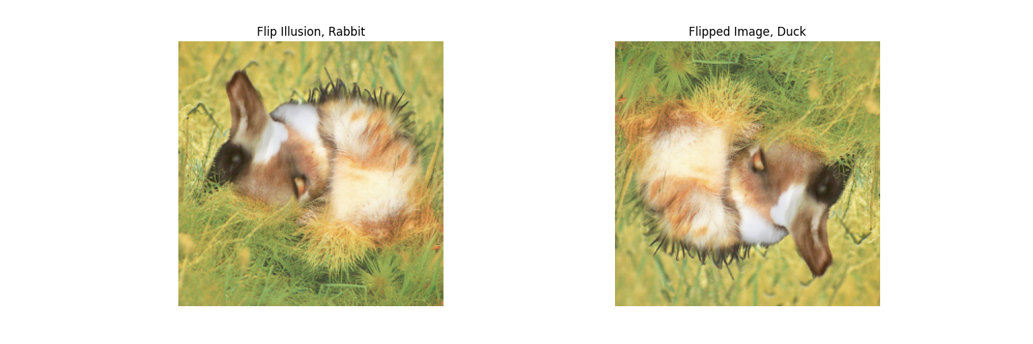
where UNet is the diffusion model UNet from before, $\text{flip}(\cdot)$ is a function that flips the image, and $p_1$ and $p_2$ are two different text prompt embeddings. And our final noise estimate is $\epsilon$. Please implement the above algorithm and show example of an illusion.
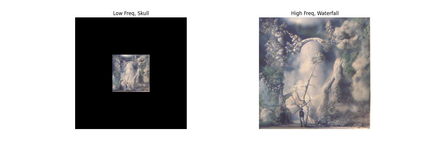
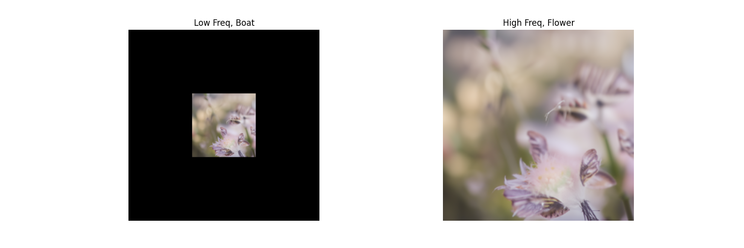
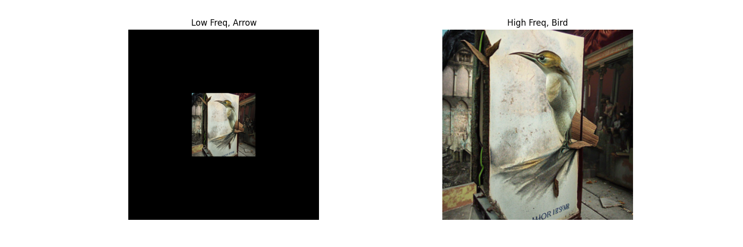
In this part we'll implement Factorized Diffusion and create hybrid images just like in project 2.
In order to create hybrid images with a diffusion model we can use a similar technique as above. We will create a composite noise estimate $\epsilon$, by estimating the noise with two different text prompts, and then combining low frequencies from one noise estimate with high frequencies of the other. The algorithm is:
$ \epsilon_1 = \text{UNet}(x_t, t, p_1) $
$ \epsilon_2 = \text{UNet}(x_t, t, p_2) $
$ \epsilon = f_\text{lowpass}(\epsilon_1) + f_\text{highpass}(\epsilon_2)$
where UNet is the diffusion model UNet, $f_\text{lowpass}$ is a low pass function, $f_\text{highpass}$ is a high pass function, and $p_1$ and $p_2$ are two different text prompt embeddings. Our final noise estimate is $\epsilon$. Please show an example of a hybrid image using this technique (you may have to run multiple times to get a really good result for the same reasons as above). We recommend that you use a gaussian blur of kernel size 33 and sigma 2.
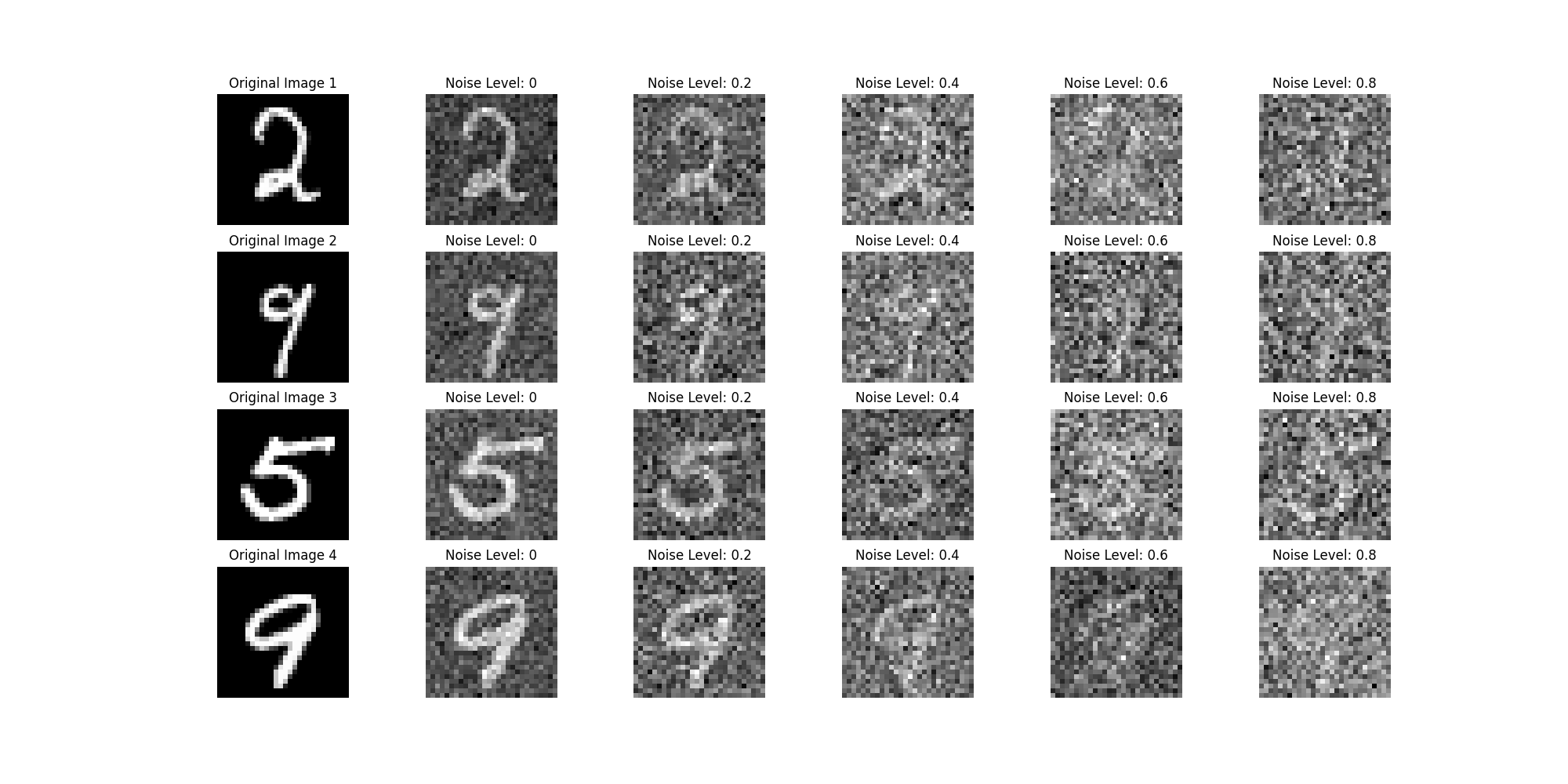
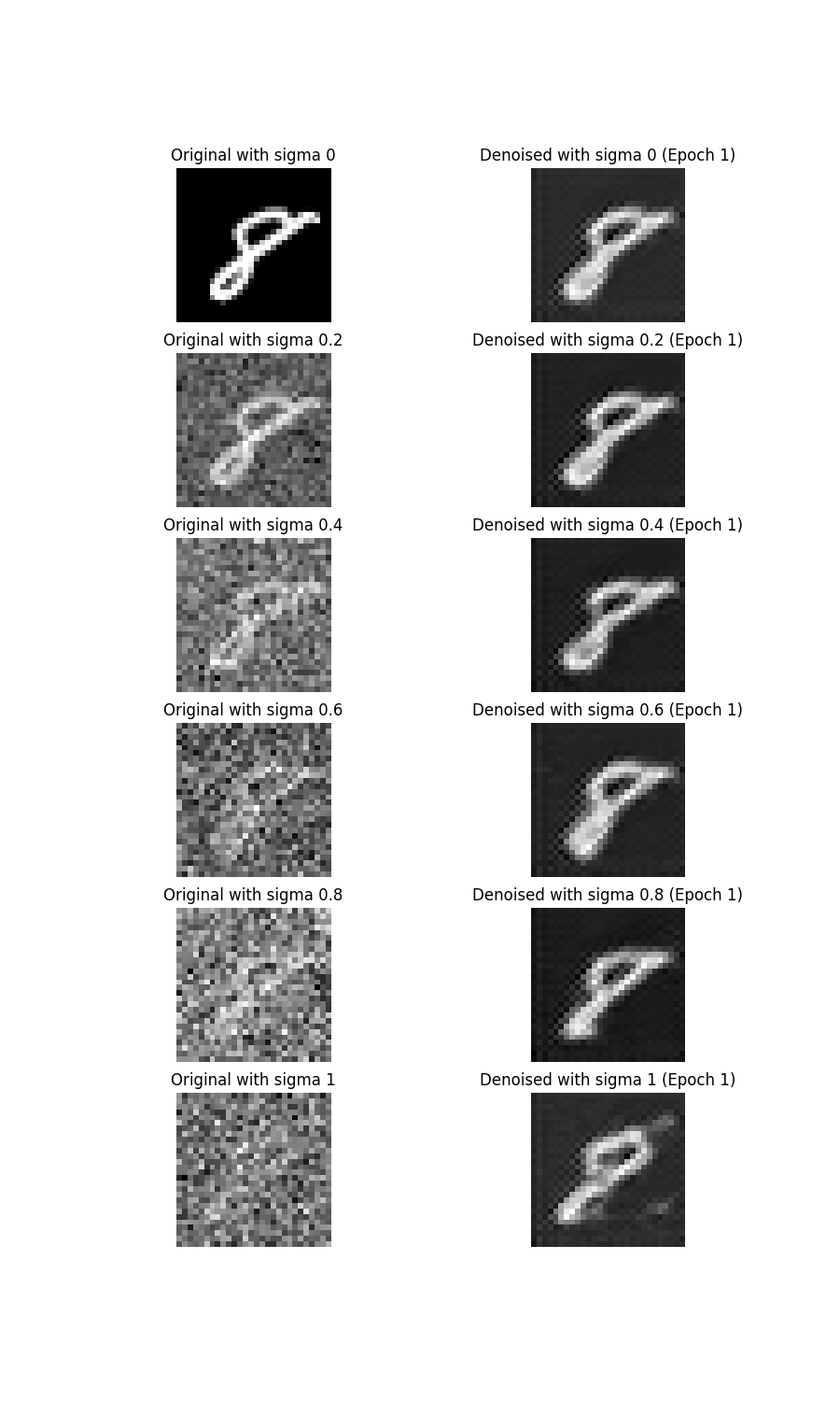
For this section, we implement a U-Net that takes in the noised image and seeks to predict the noise from the original, clean image. Below we first visualize the effect of $\sigma$ on adding noise to the image.
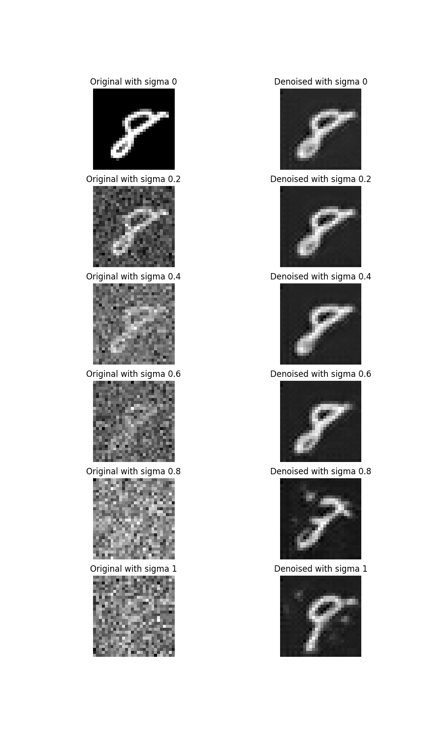
In this part, $\sigma = 0.5$ for all the training set, so the model only sees a single sigma. We observe that the loss quickly reduces in the first few epochs, and levels off at around 0.01.
Even though the model has only been trained on $\sigma = 0.5$, it is remarkably competent at denoising $\sigma < 0.5$, and was somewhat capable of $\sigma = 0.6$, but the modality collapses at higher noise levels. In this instance, the number 8 was de-noised into the number 9, which suggests that the model has learned some manifold of the MNIST digits.
In this section, we first implement a U-Net that is only dependent on the time (from a time-based noise schedule), and independent of the class.
We first plot the loss curve, and we observe that the loss decreases rapidly and levels off at around 0.02. There is a spike near the end of training, possibly due to some instability with learning rate schedules but it quickly drops off again.
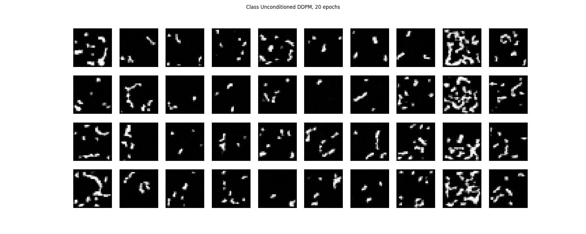
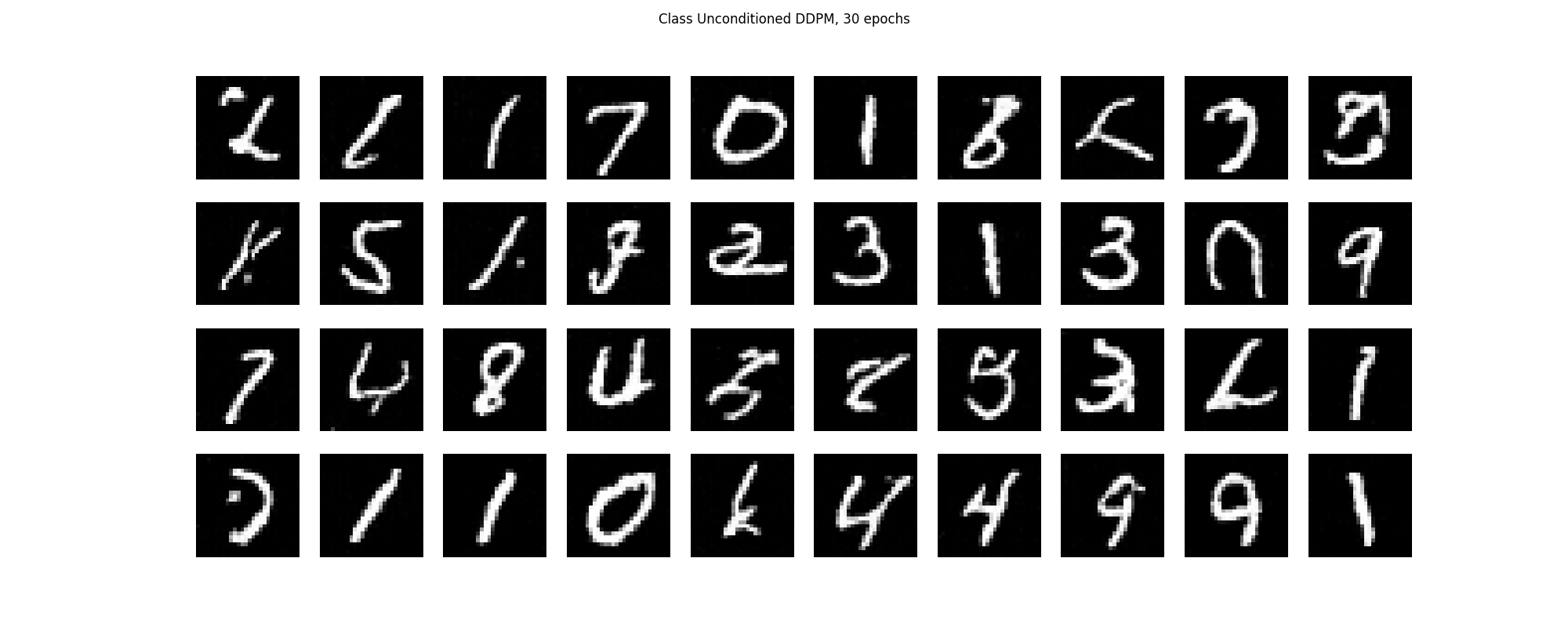
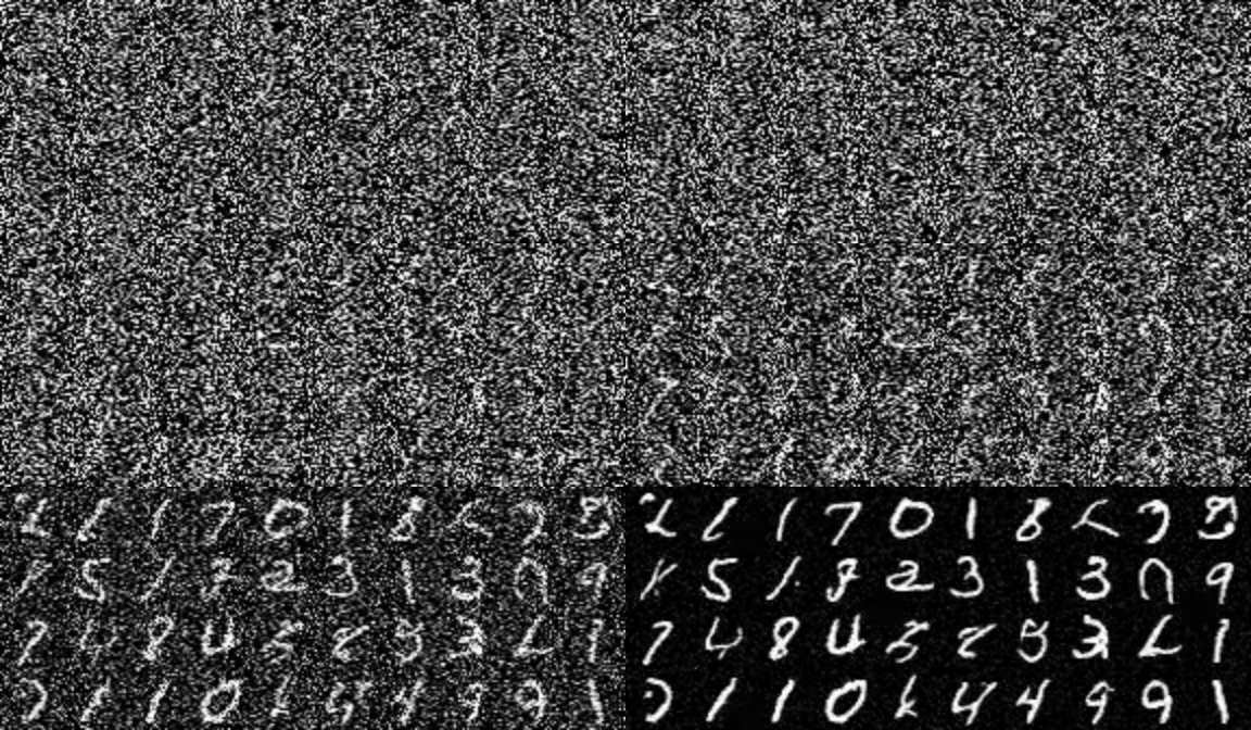
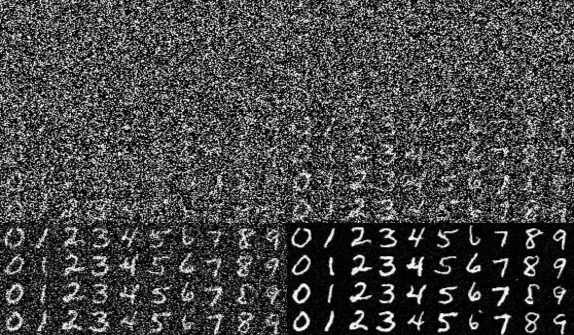
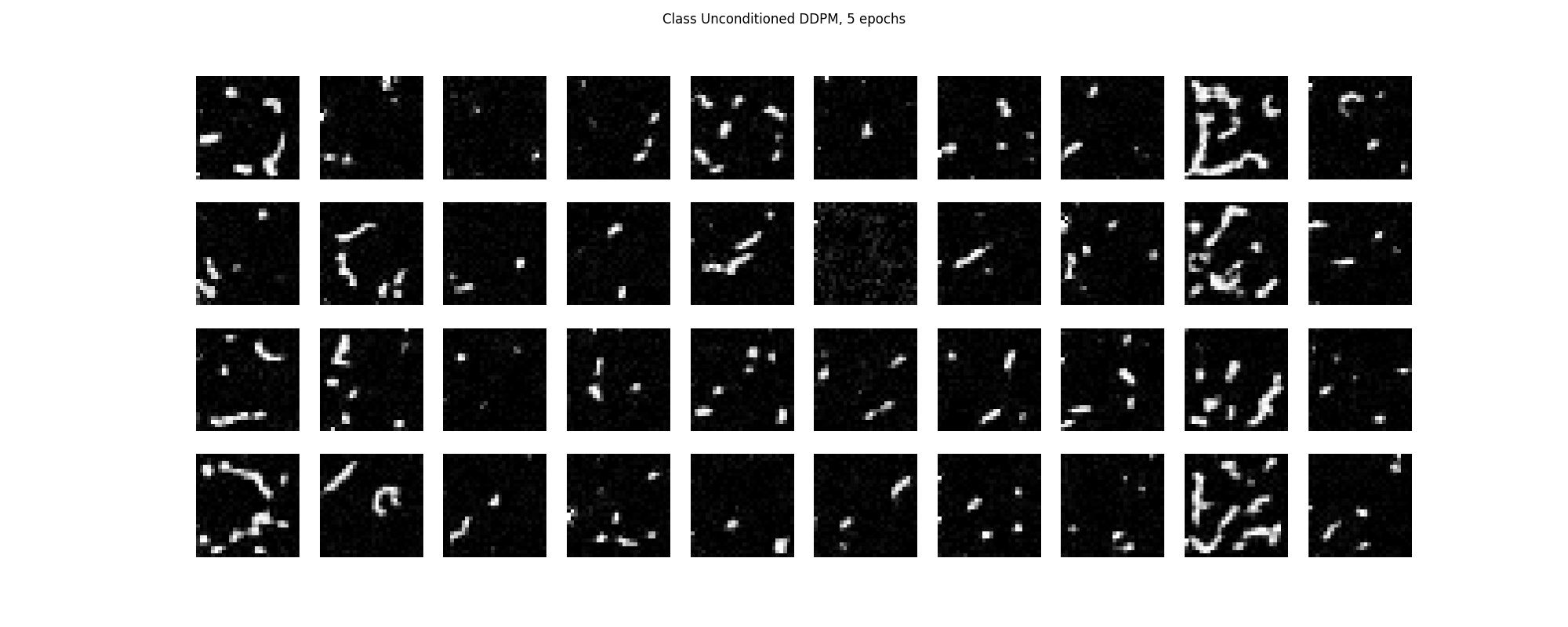
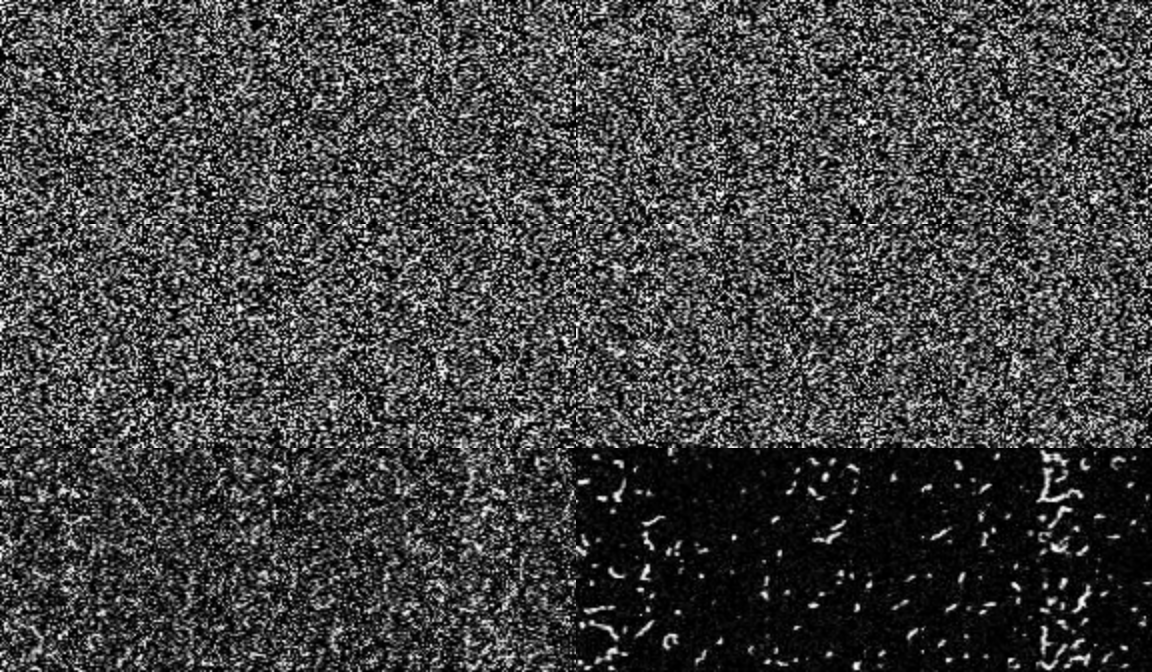
Below we sample from the network 40 times, and we also show videos showing the denoising process at different training epochs.
After 5 epochs, we observe that the model seems to have learned a correct distribution of black/white pixels, but they are randomly scattered around the image.
After 20 epochs, we observe that the model has learned rudimentary strokes, but they are again scattered and do not have any structure.
After 30 epochs, we observe that the model has learned some understanding of the digits and images are somewhat coherent. Most generations are digits or could conceivably have been digits if humans chose different symbols thousdans of years ago.
In this section, we first implement a U-Net that is dependent on both the time (from a time-based noise schedule) and independent the class (what digit).
We first plot the loss curve, and we observe that the loss decreases rapidly and levels off at around 0.02. There are a few spikes during training, possibly due to some instability with learning rate schedules but it quickly drops off.
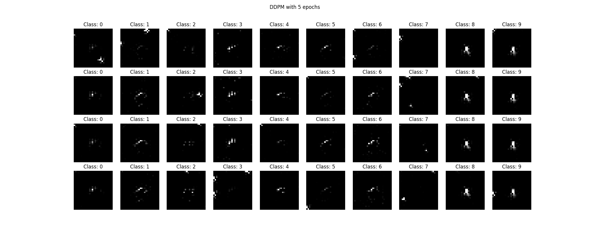
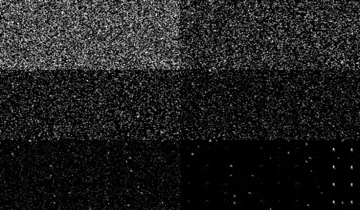
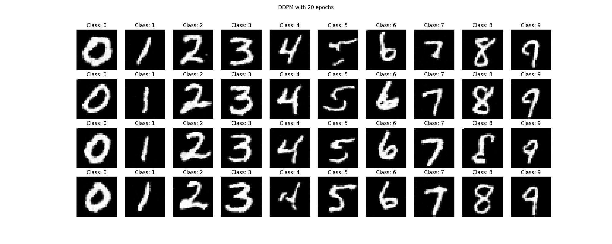
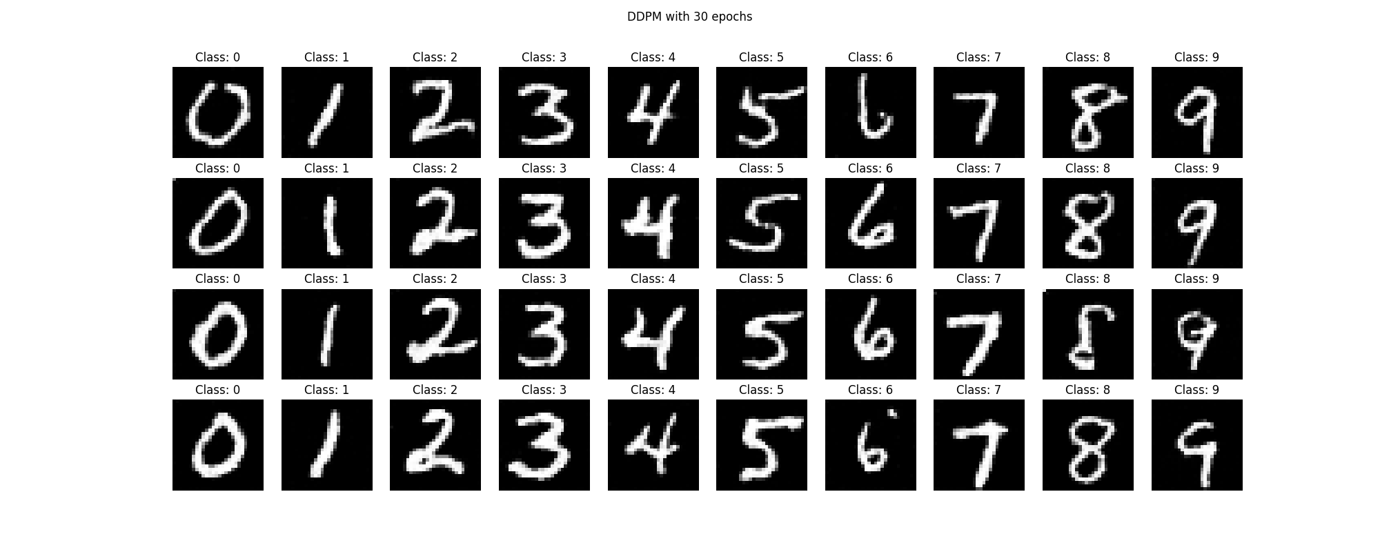
Below we sample 4 times for each of the 10 digits, and we also show videos showing the denoising process at different training epochs.
After 5 epochs, we observe that the model has not learned any significant understanding of the digits, but the background is mostly dark and noiseless.
After 20 epochs, we observe that the model has learned the digits very reasonably, but there is still some noise that persists.
After 30 epochs, we observe that the model has slightly improved over the 20 epoch version, with overall less noise in the final image.