2. Recover Homographies
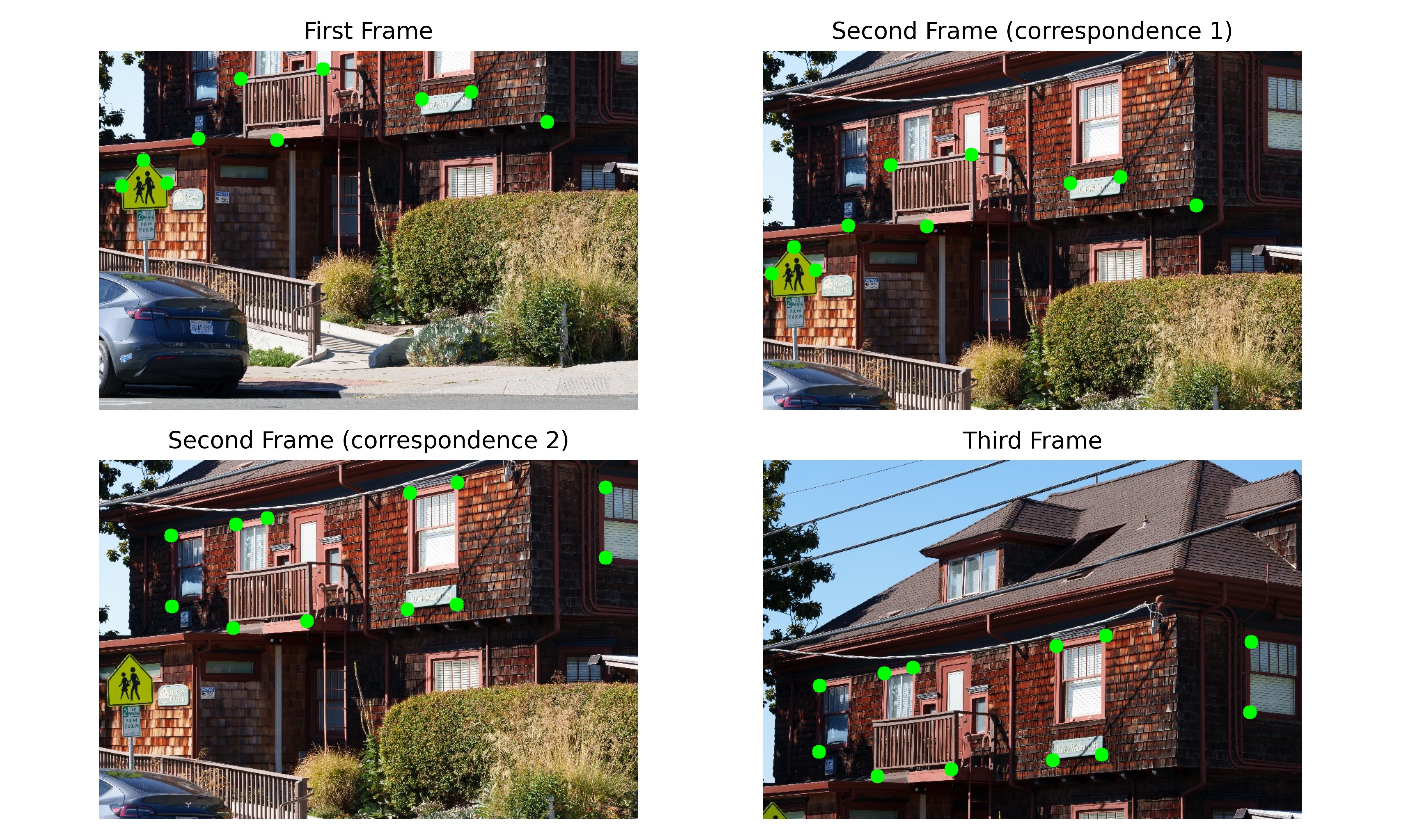
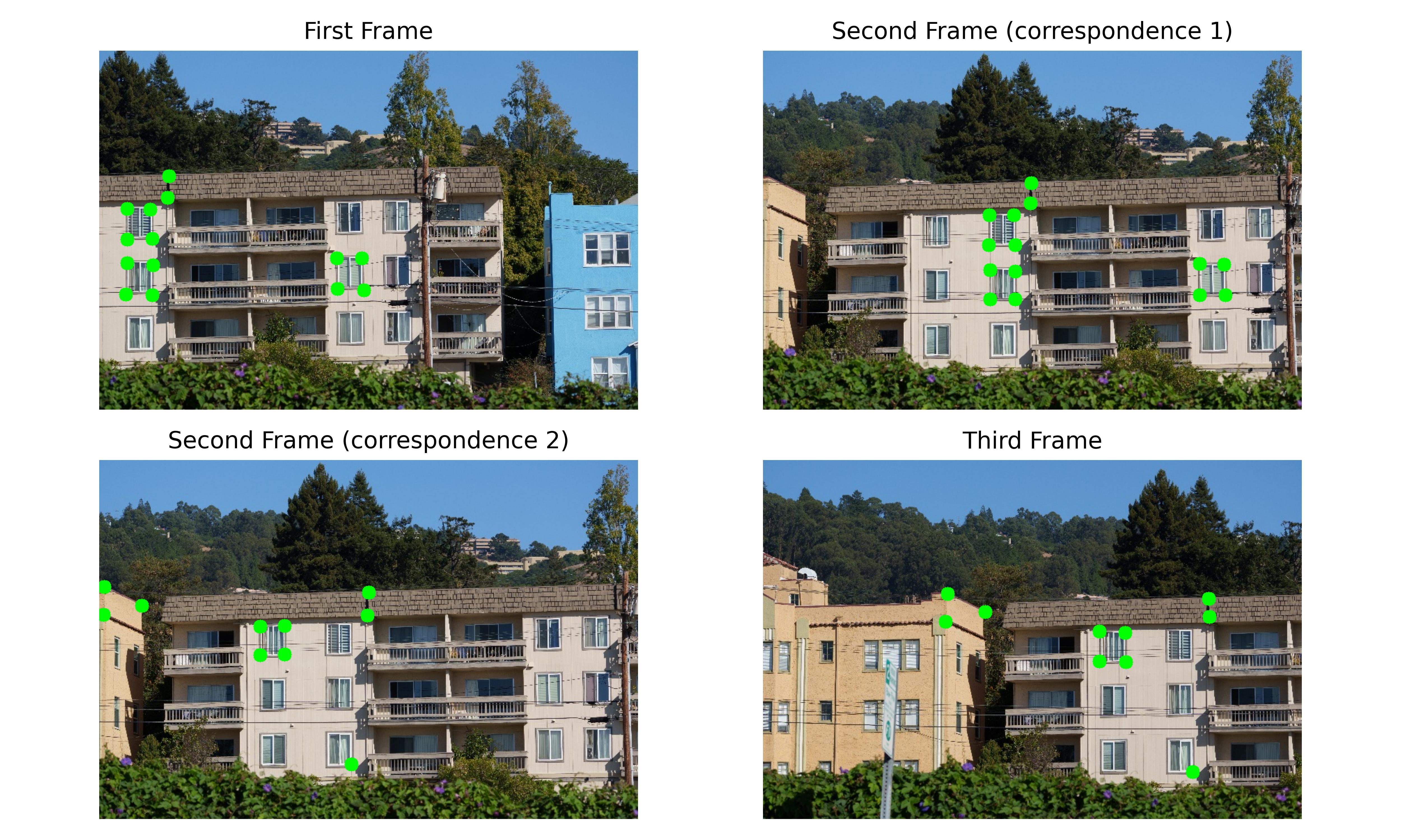
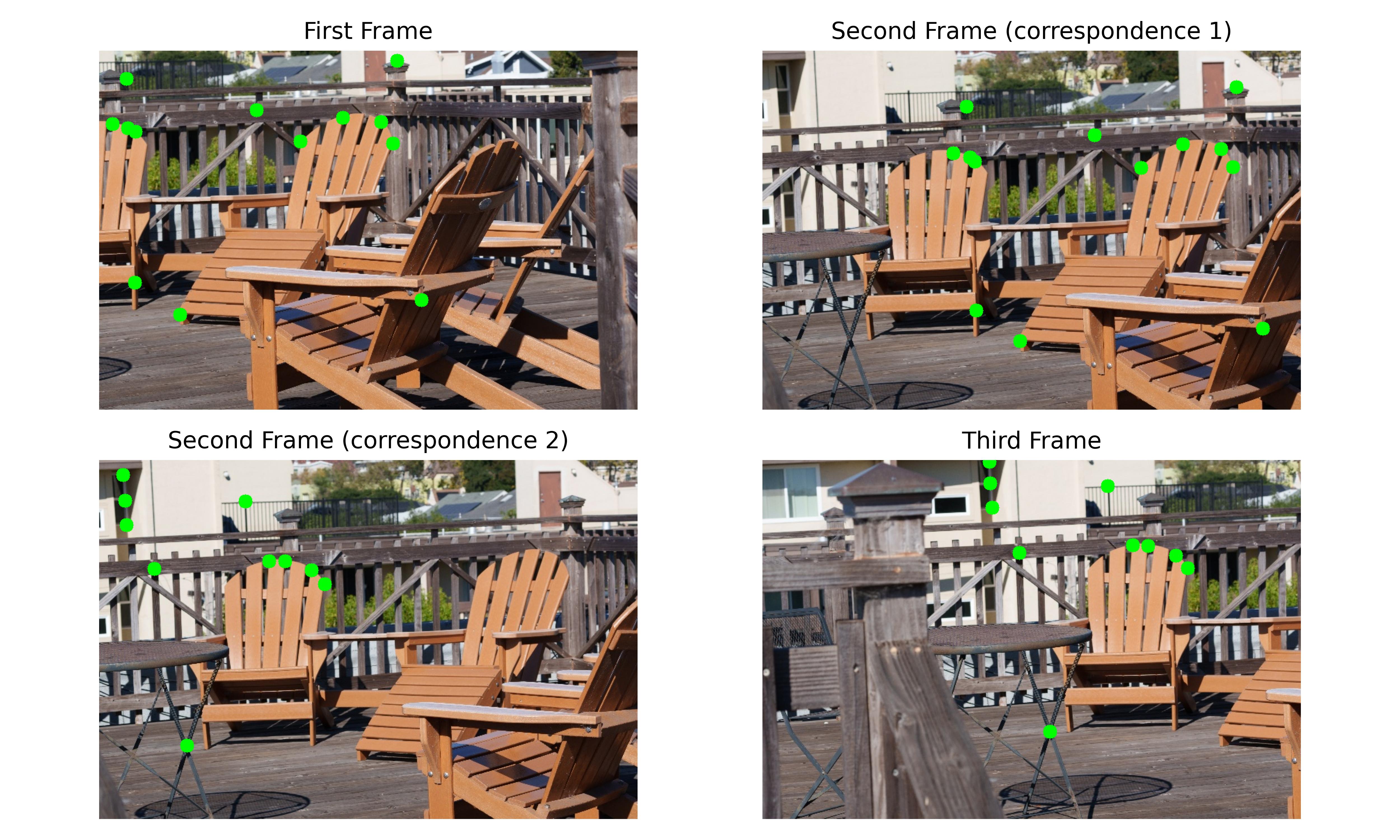
We manually label corresponding points using the tool we developed in Project 3.
We present the images and the labels below.
# Set up
import cv2
import numpy as np
import os
import scipy.signal
from tqdm import tqdm
from matplotlib import pyplot as plt
import matplotlib
import cowsay
from glob import glob
import scipy

matplotlib.rcParams["figure.dpi"] = 500
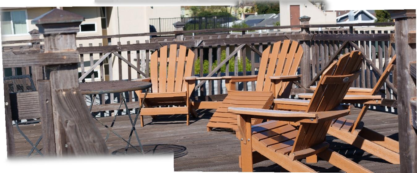
The photos are captured on a Sony A6700 at the 70mm (105mm equiv) focal length. Images are straight out of camera and downsampled to accelerate computation time.
We manually label corresponding points using the tool we developed in Project 3.
We present the images and the labels below.
Given these correspondences, we can estimate the transform between the two images with $$ \begin{bmatrix} wx' \\ wy' \\ w \end{bmatrix} = \begin{bmatrix} a & b & c \\ d & e & f \\ g & h & 1 \\ \end{bmatrix} \begin{bmatrix} x \\ y \\ 1 \end{bmatrix} $$
Plugging it into a symbolic calculator we have $$ \begin{bmatrix} x' \\ y' \end{bmatrix} = \begin{bmatrix} x & y & 1 & 0 & 0 & 0 & -xx' & -yx' \\ 0 & 0 & 0 & x & y & 1 & -xy' & -yy' \\ \end{bmatrix} \begin{bmatrix} a \\ b \\ c \\ d \\ e \\ f \\ g \\ h \end{bmatrix} $$
Since we have more than 4 correspondences, we have an overconstrained system, so we estimate the matrix using least squares.
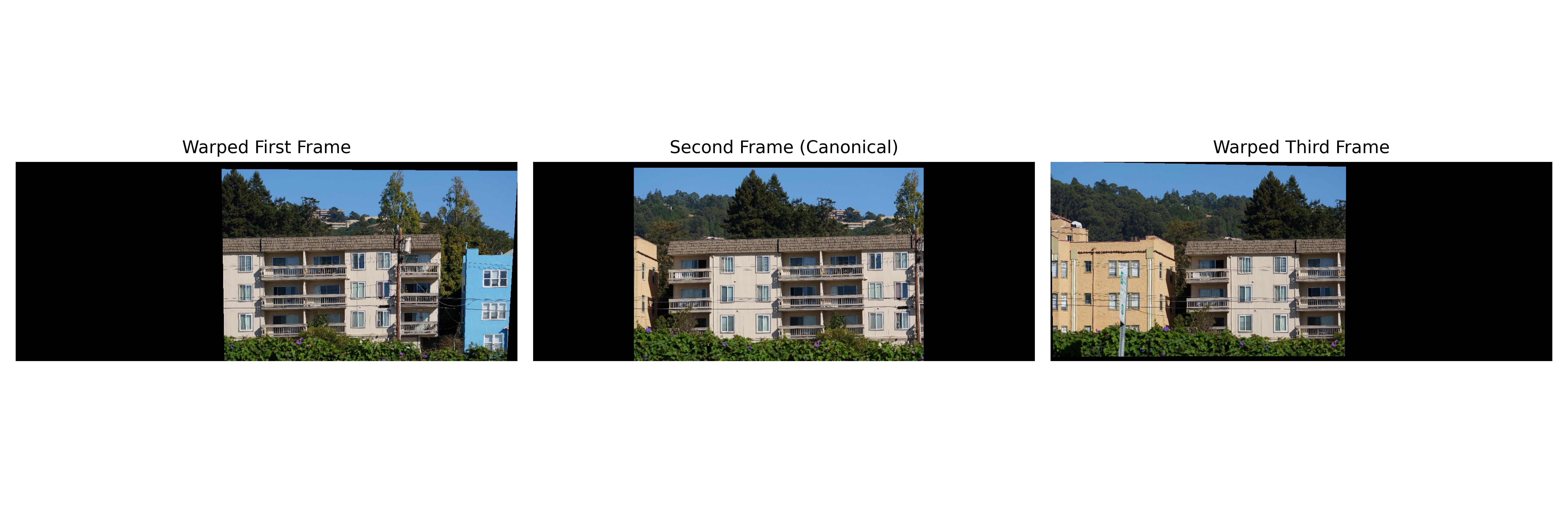
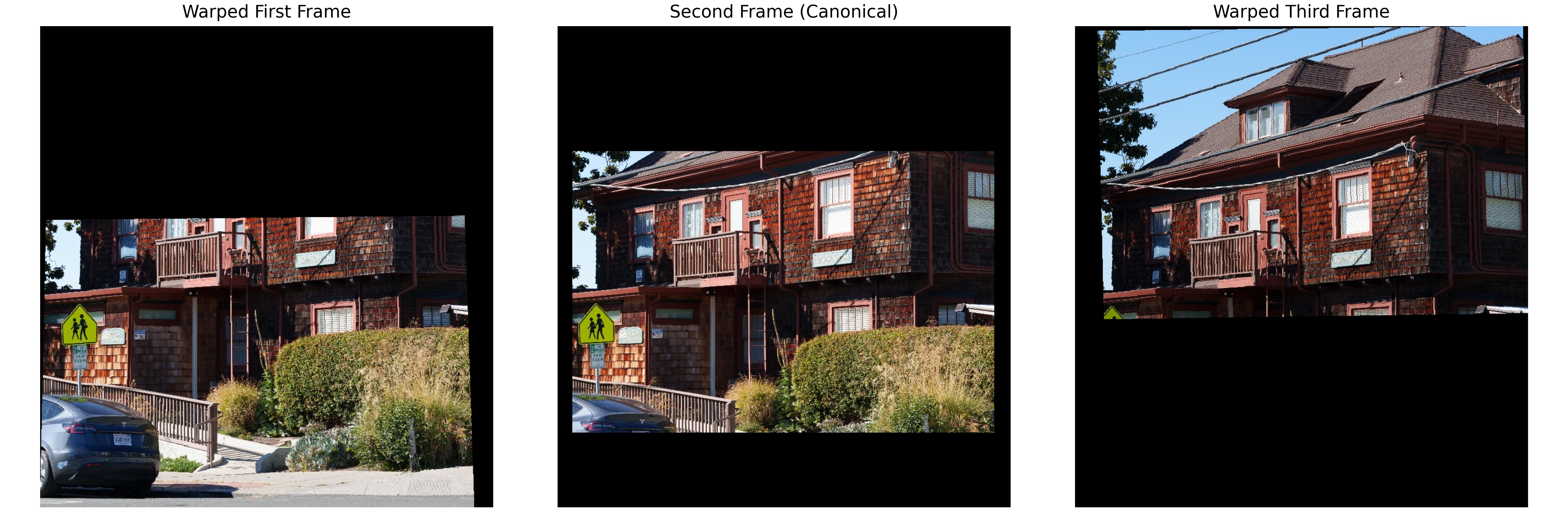
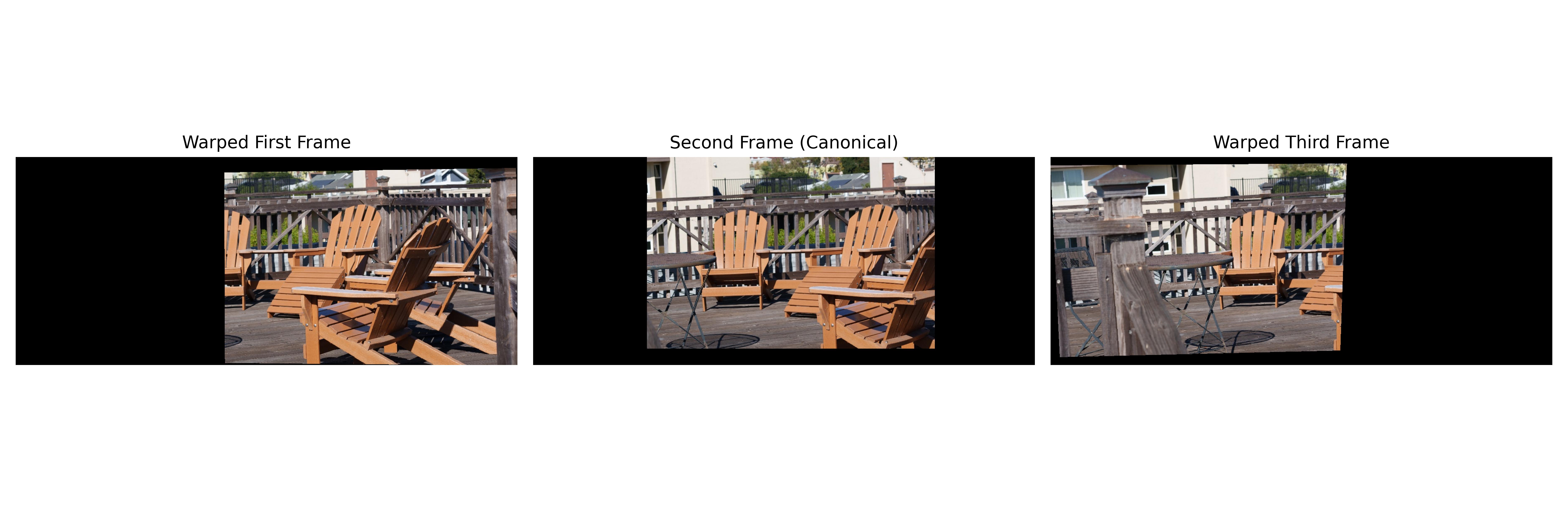
We modify the warp function that we developed in Project 3 to allow for more pixels. Namely, we compute the locations of the corners, and shift them so they are positive and well defined in image space. Then we compute the inverse transform to retrieve the images. At this step, we compute the image cordinates of all images in our chosen canonical center. This way, we do not have to worry about relative translations after the warp.
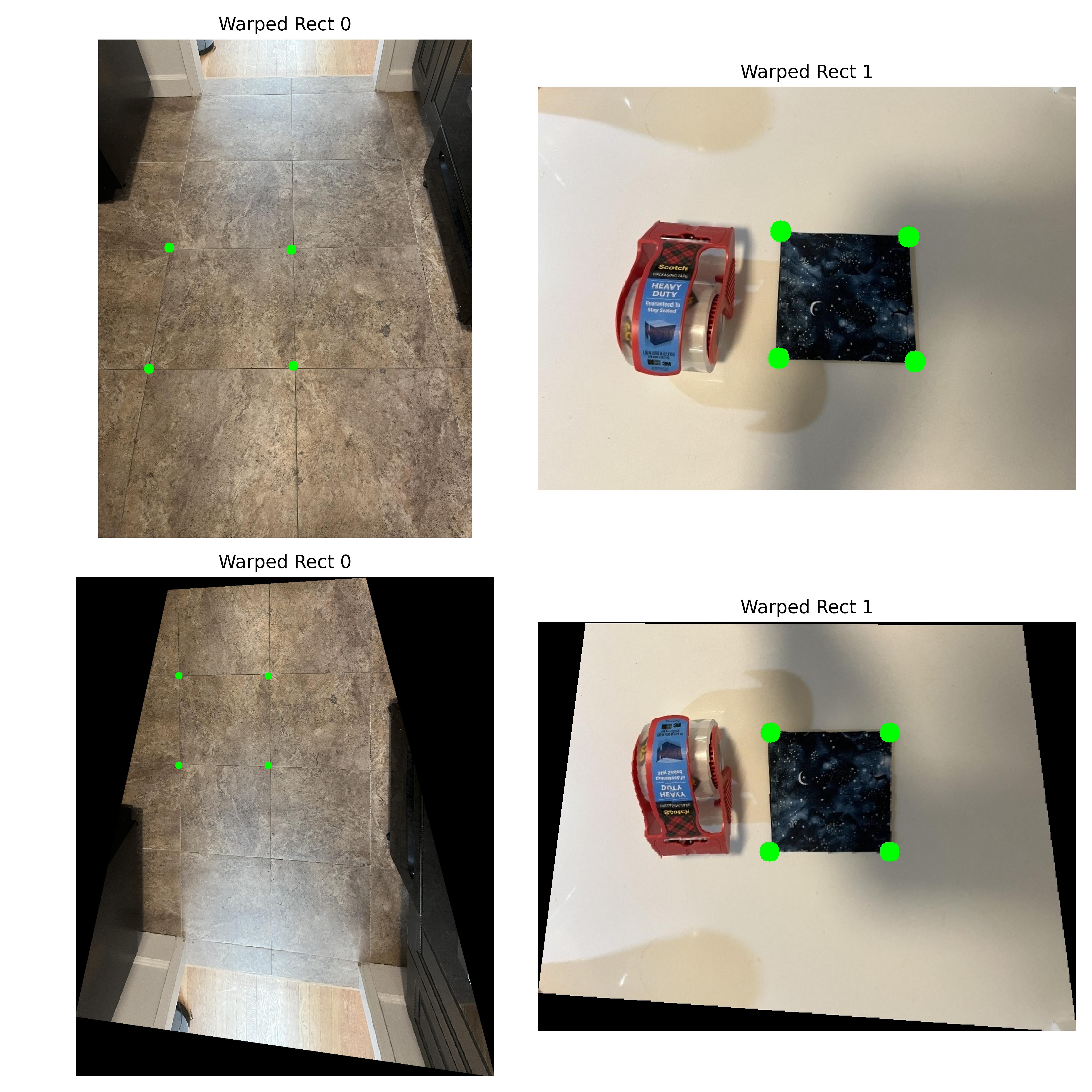
Take a photo containing paintings, posters, or any other known rectangular objects and make one of them rectangular - using a homography. In this section, we demonstrate the correct working of our implementation by rectifying 2 square shapes: the tile of the floor and the shape of a square cloth coaster.
We observe that this creates a lot of artifacts. For example, the pedestrain sign is misaligned for the first image and the chair's are misaligned in the last one. We then seek to improve the results with alpha blending. This method makes the alpha value smaller towards the edges so there is less of a hard barrier between images. We observe significant improvements to the barrier problem,but there is a lot of ghosting due to slightly misalighted images.
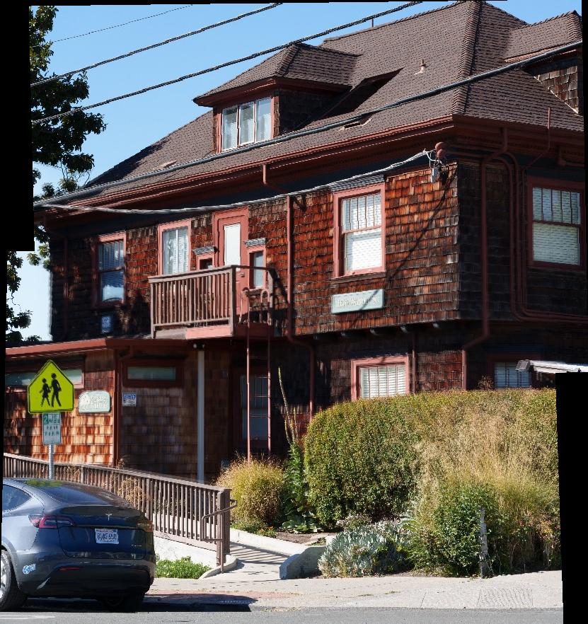
To address the ghosting issue, we use lapachian blending. By blurring the image's edges, we seek to relieve both the edge issue and the ghosting issue at the same time.
We see that the results are much better. The artifcats are more blurred and there is no visible ghosting. One interesting thing to note is that these mosaics are significantly less perspective warped than the sample's. An explanation might be the 105mm equivalent focal length. Since my lens is more zoomed in, the images taken with them would take up less space on the project sphere, thus there is less persective warping even though I turned the camera quite a bit to capture a larger scene.
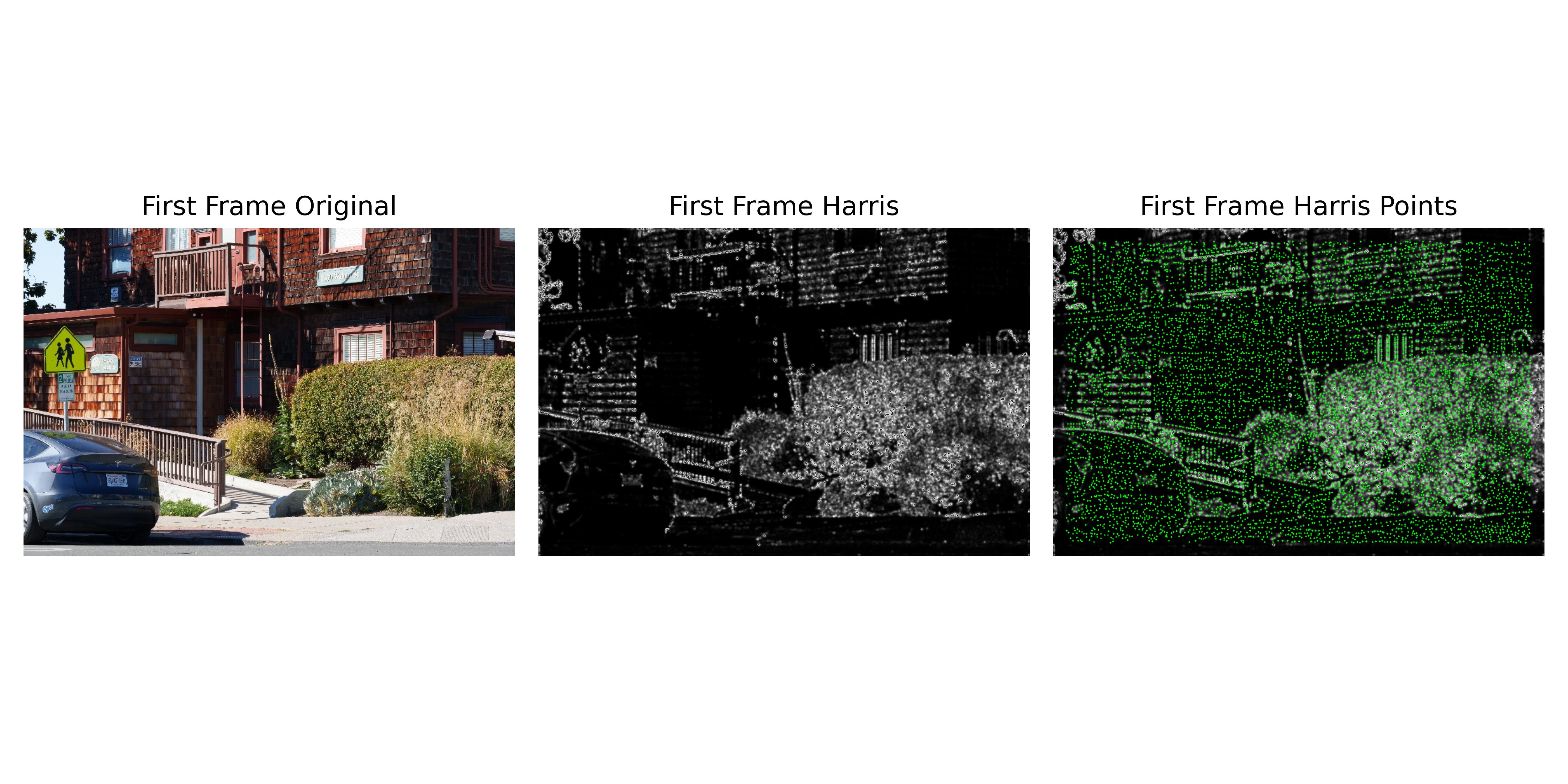
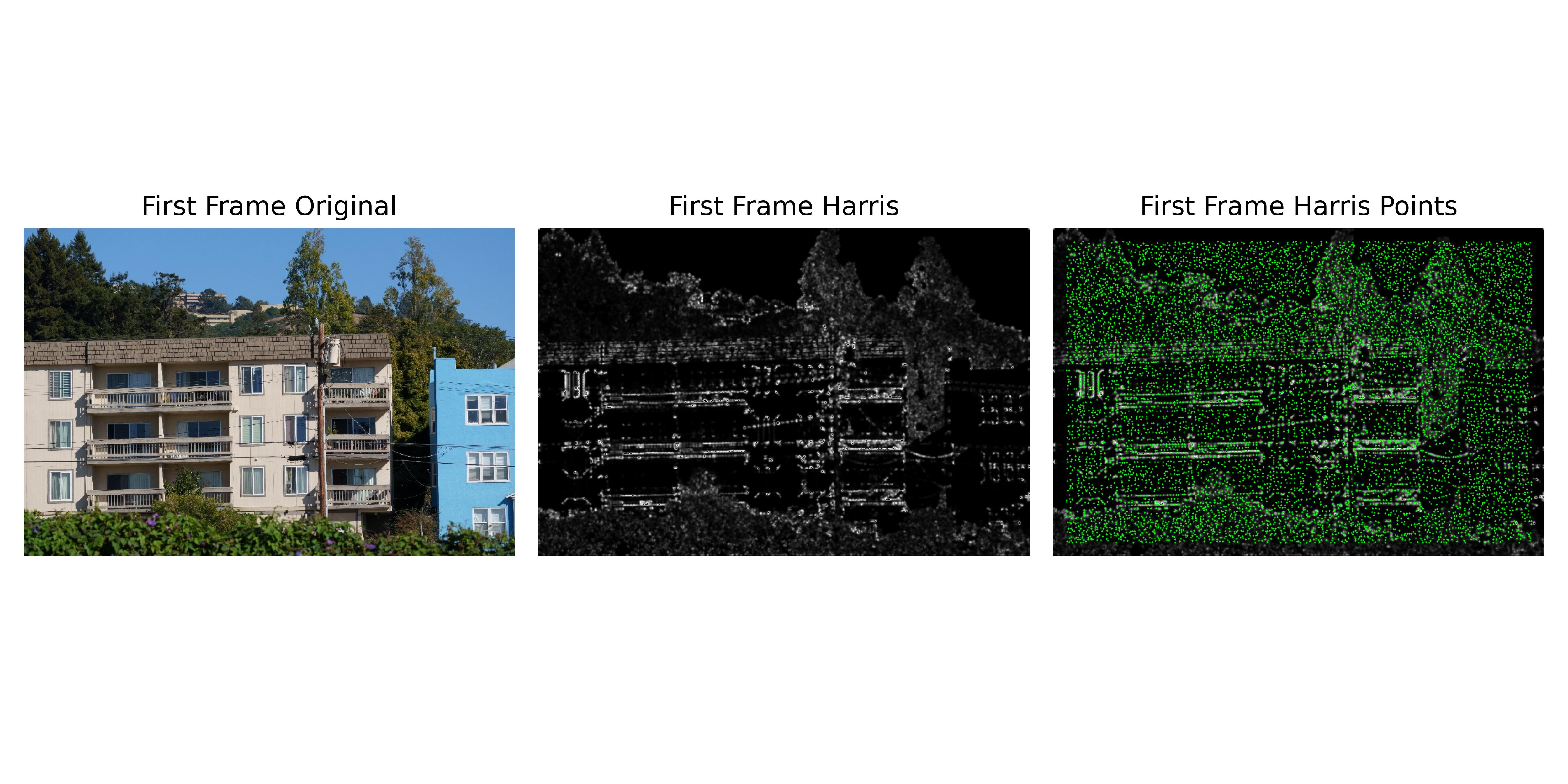
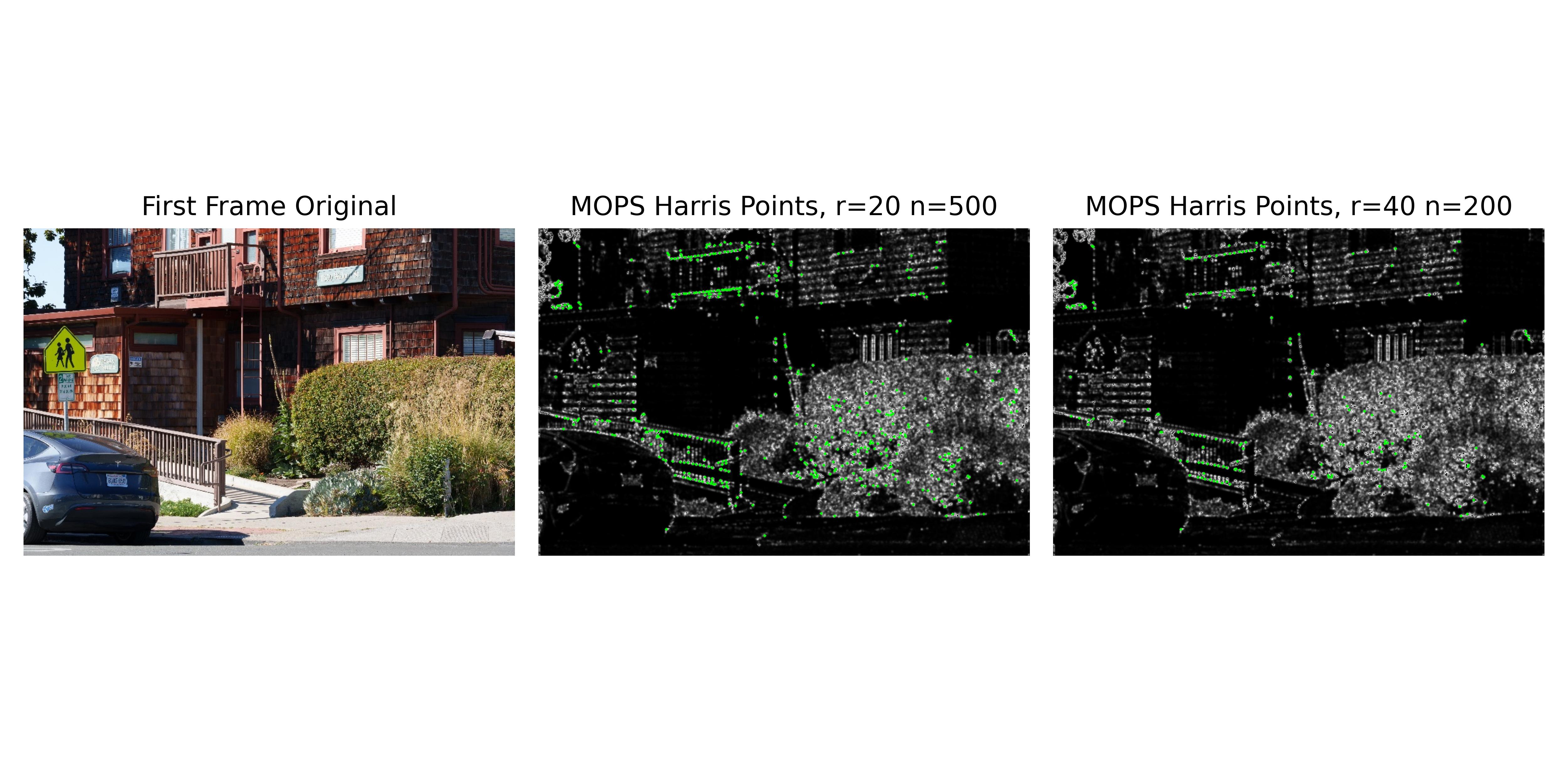
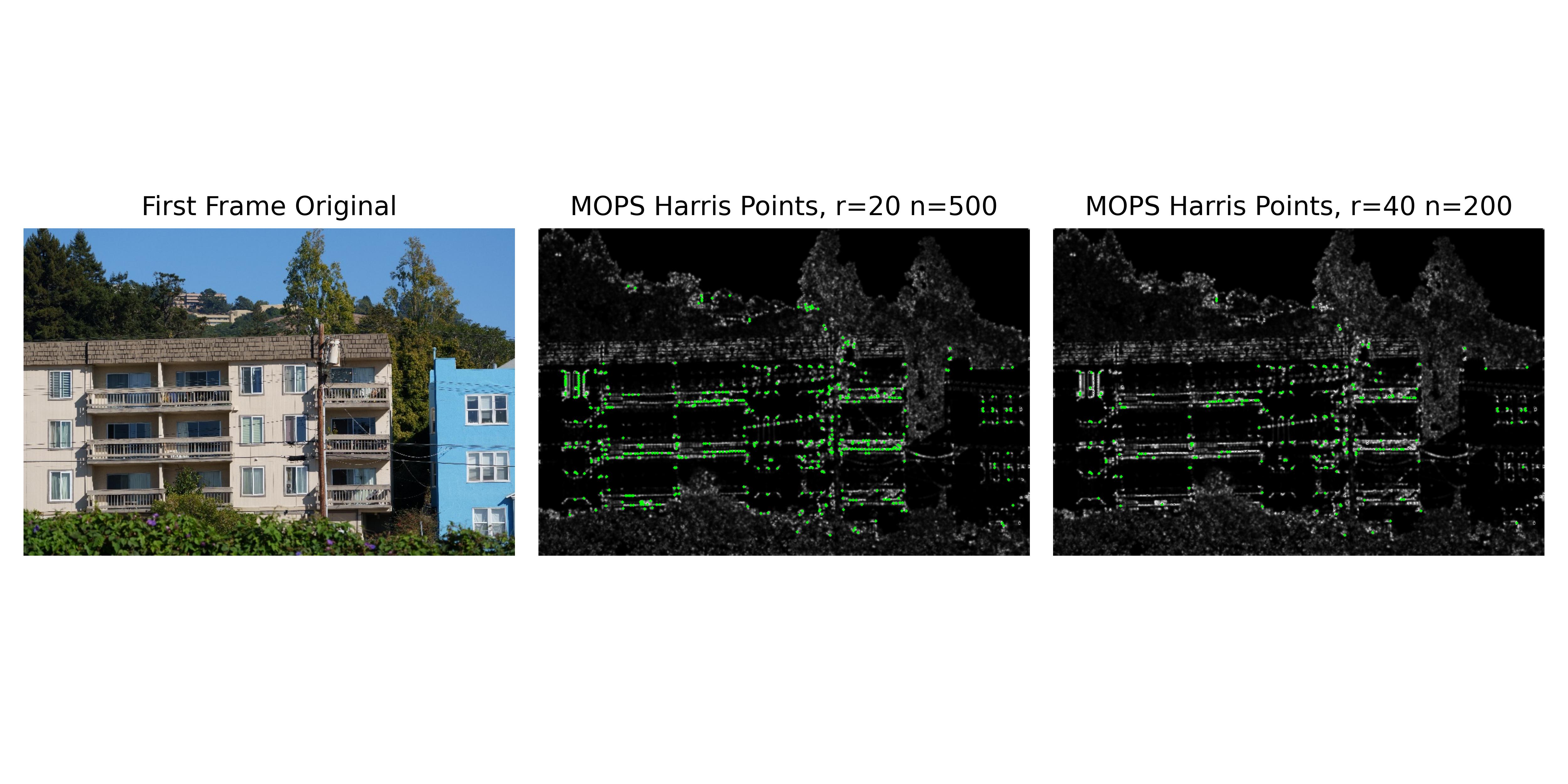
To enable automatic stitching, we first extract features from each of our images. To do this we use the Harris Corner detector. This detects corners by measuring the gradient in the x and y directions.
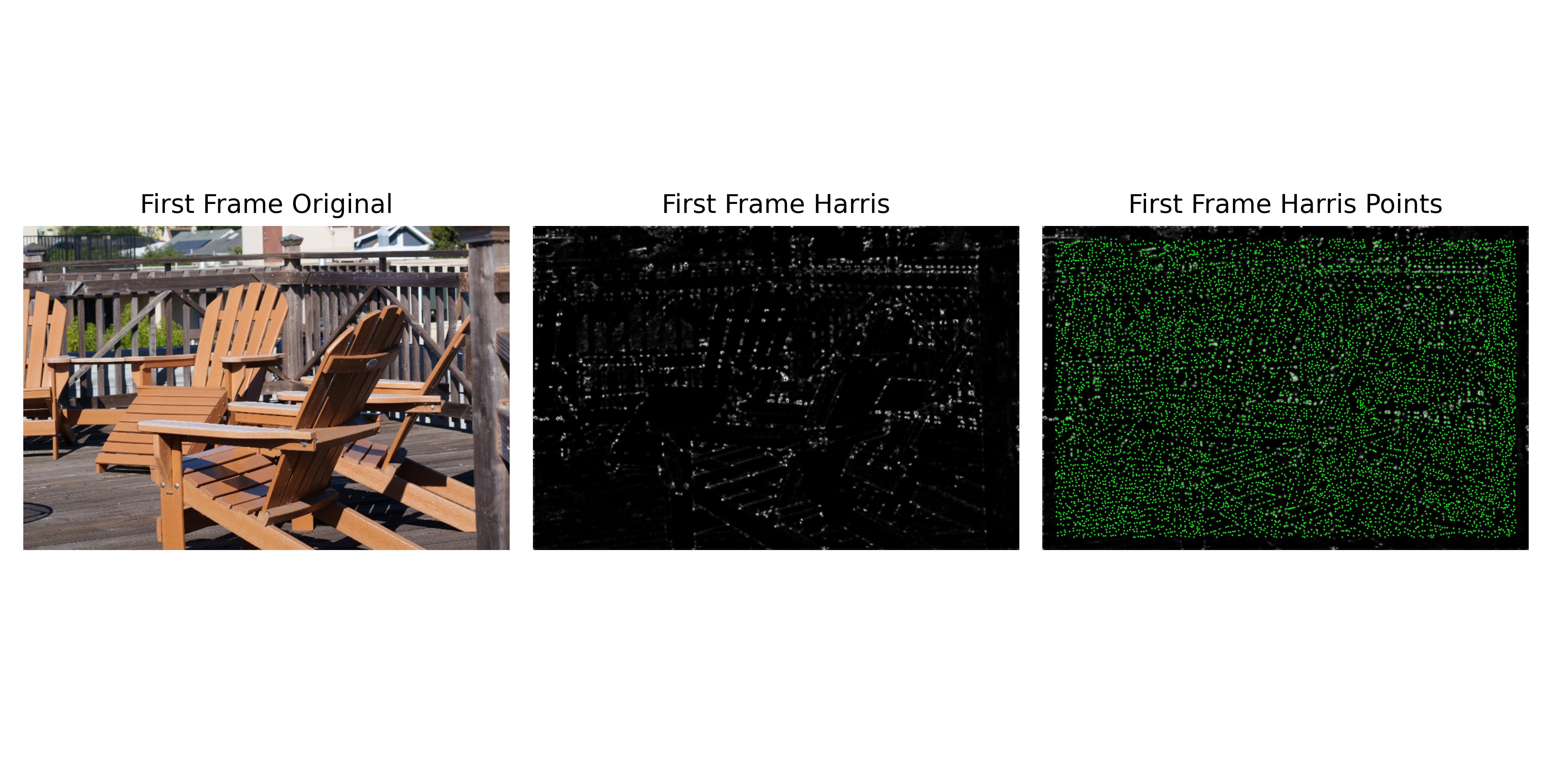
There are too many points in this example, so we need to downsample. We use the ANMS technique, and reduce the number of points to a fixed amount. Below we compare the results of sampling 200 points with a radius of 40 and sampling 500 points with a radius of 20.

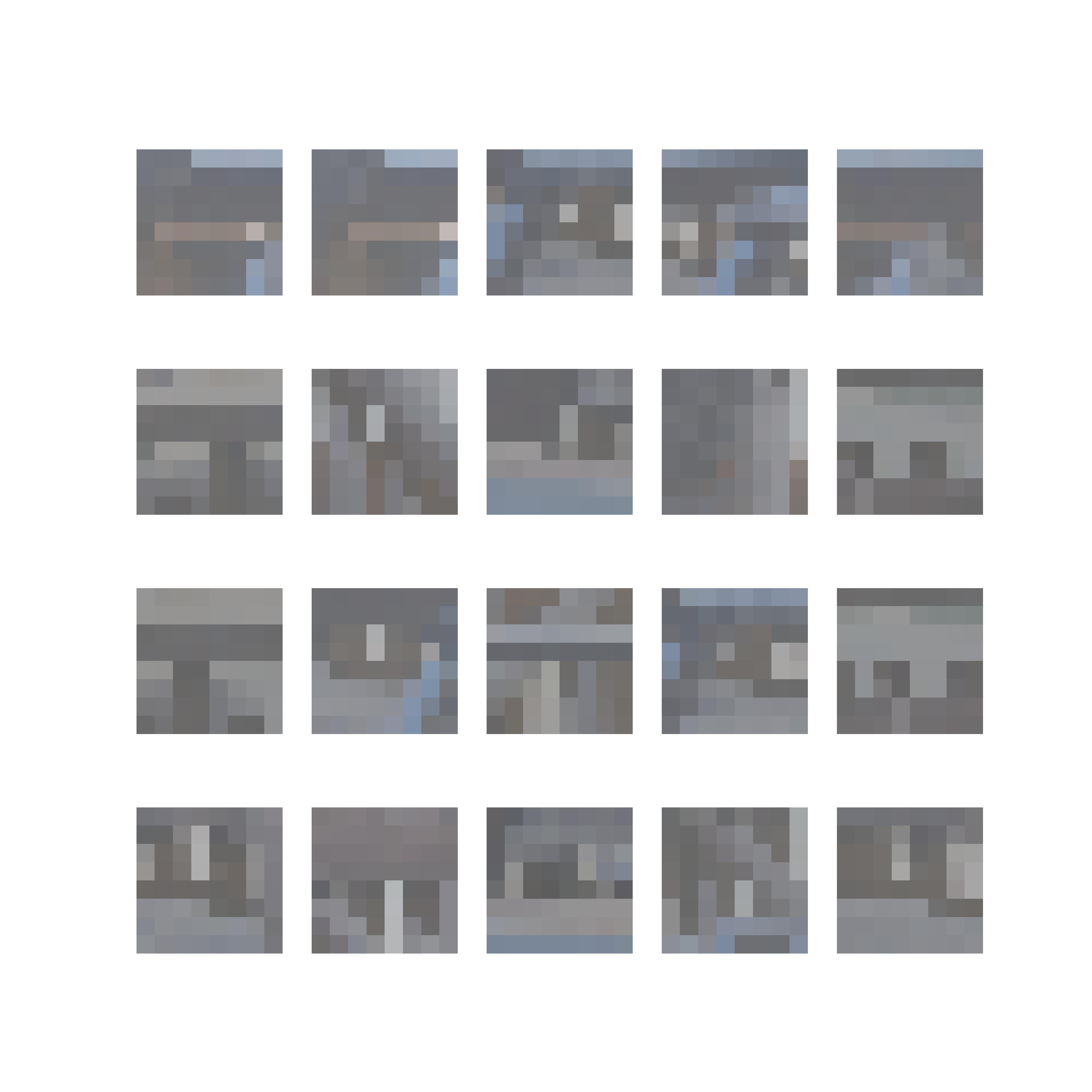
We compute the MOPS patches, which are 40x40 patches extracted with the center at the filtered Harris Points above. We then downsample these patches to 8x8 descriptors. Below we visualize a few patches from the chair scene.
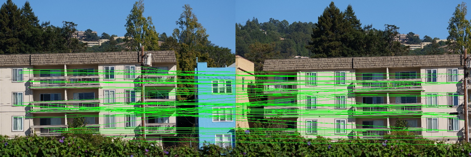
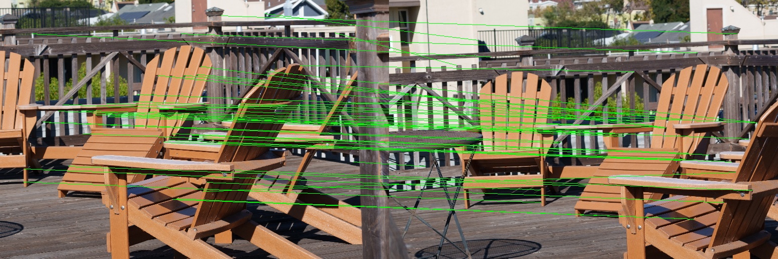
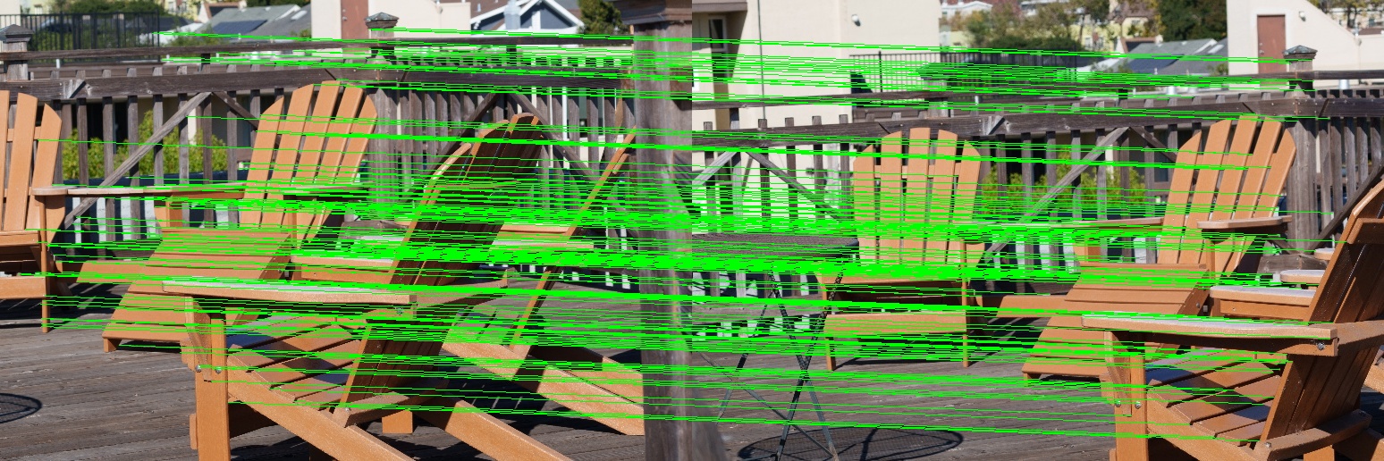
To match these patches to each other, we use Lowe's trick. We apply a threshold (0.85) between the difference with the nearest neighbor and the difference with the second nearest neighbor. The motivation is that if a patch exists in both frames, then it should have 1 unique nearest neighbor. We visualize the matches below.
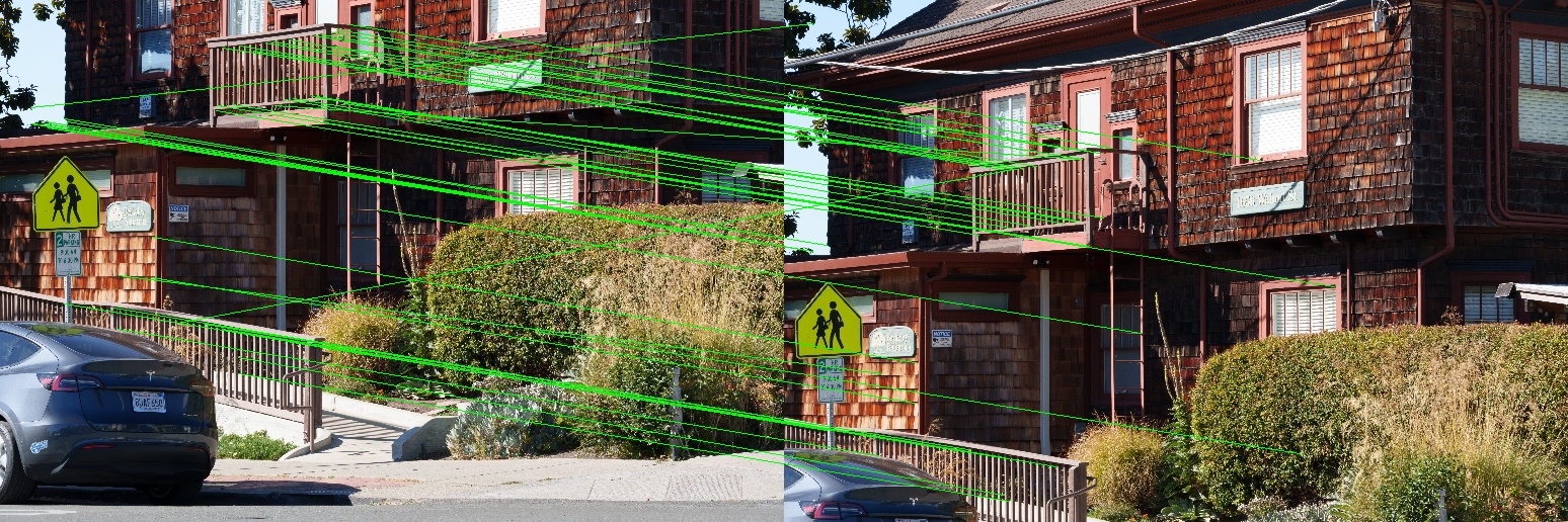
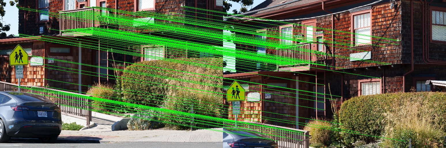
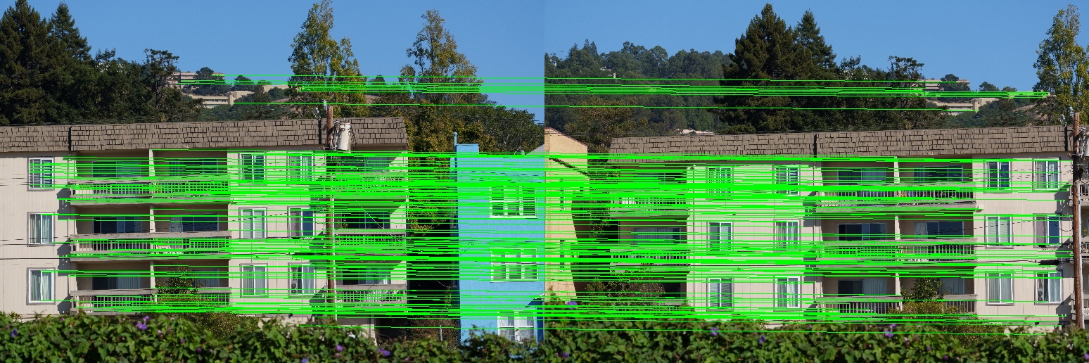
We notice that although most of the correspondences are correct, a lot of them are not. We then seek to reject outliers using RANSAC. We implement it by warping the Harris points with the proposed transformation $h$. We use 1000 iterations and a threshold of 1. Below we visualize the RANSAC matches. We can see that all the correspondences agree with each other.
Finally, we visualize the results of the hand labelled images and the automatically stitched ones. All blending techniques are the same.
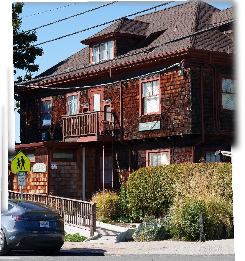
Below is the manually labelled brick scene.
Below is the automatically stitched brick scene.

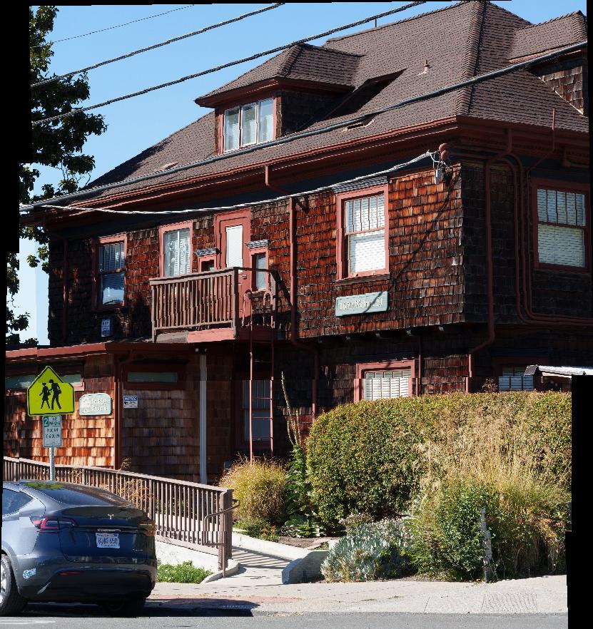
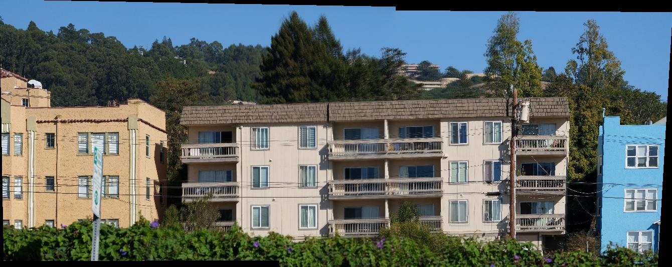
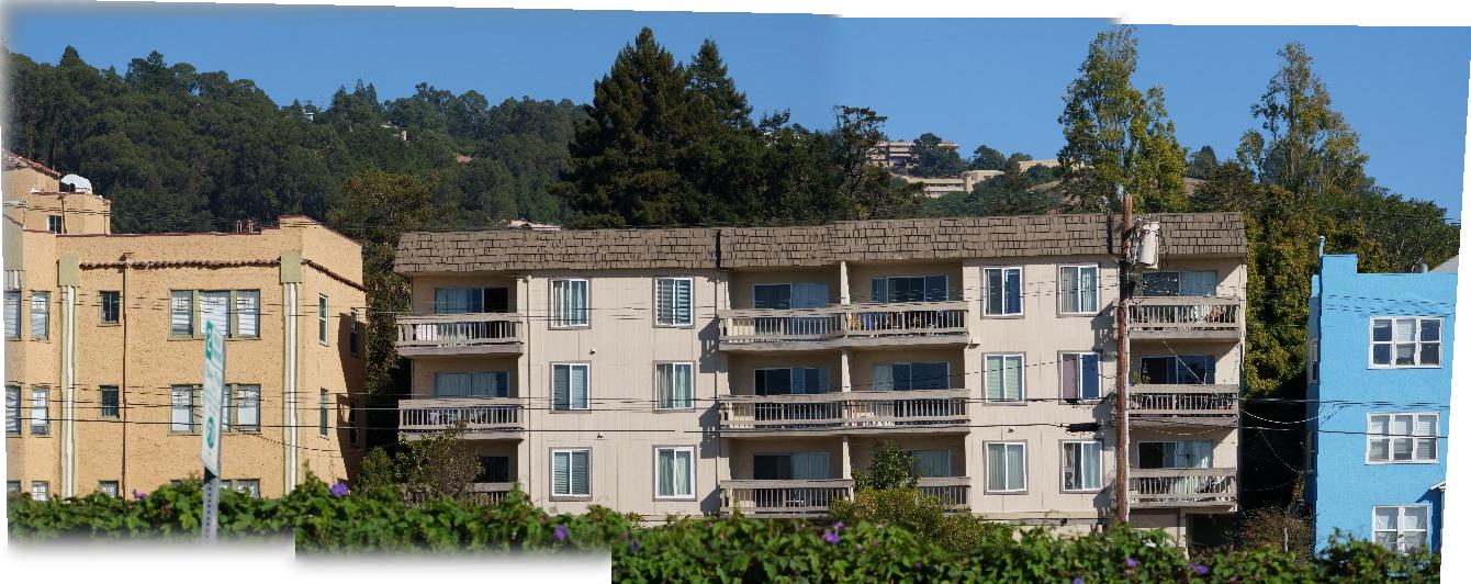
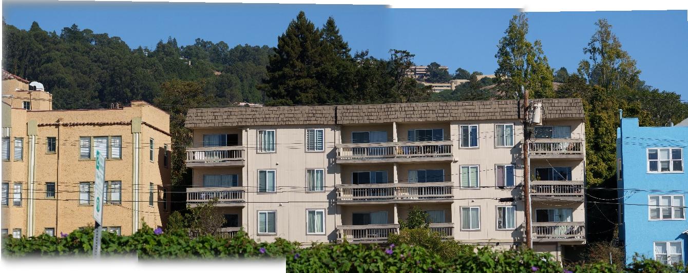
Below is the manually labelled building scene.
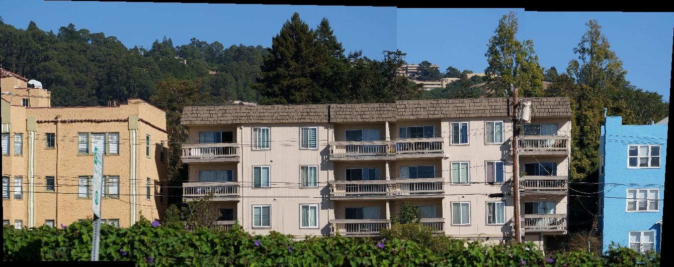
Below is the automatically stitched building scene. Notice the smoother roof on the right side.
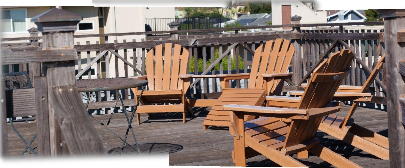
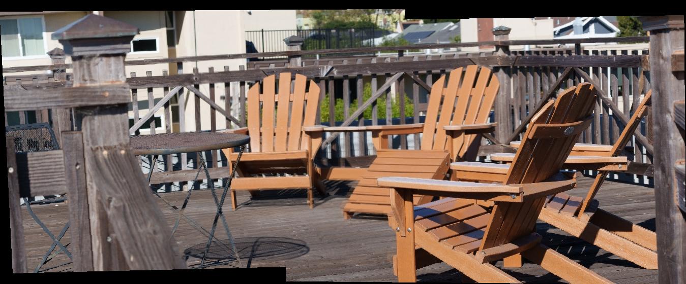
Below is the manually labelled chair scene.
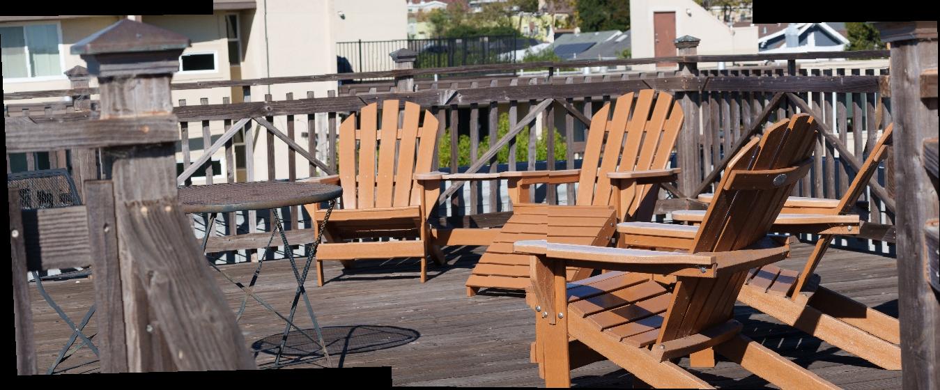
Below is the automatically stitched chair scene. Notice the smoother edge of the chairs on the right side.